set.seed(30)
class_size <- 25
birthdays <- sample(1:365, class_size, replace = TRUE)
sort(birthdays)
[1] 1 10 29 35 41 96 110 116 140 154 188 193 209 253 269 281 301 304 305
[20] 305 306 315 324 330 330Before any code: go around the room and say your birthday (month and day only). Did two people match?
That’s one experiment, and it gives one yes-or-no answer. It can’t tell us the chance of a match, any more than one random walk could tell us the typical distance. For that, we need many rooms.
We’ll make the same simplifying assumptions the classic version of this problem makes:
R’s sample() draws values at random from a list. sample(1:365, 25, replace = TRUE) picks 25 days of the year, and replace = TRUE lets the same day be picked more than once, which is exactly what a shared birthday is. Like runif(), sample() gives every choice an equal chance.
set.seed(30)
class_size <- 25
birthdays <- sample(1:365, class_size, replace = TRUE)
sort(birthdays) [1] 1 10 29 35 41 96 110 116 140 154 188 193 209 253 269 281 301 304 305
[20] 305 306 315 324 330 330Each number is a day of the year: 1 is January 1, and 365 is December 31. Sorting makes matches easy to spot. Do you see any?
duplicated() marks each value that already appeared earlier in the list, and any() asks whether at least one is TRUE:
any(duplicated(birthdays))[1] TRUEbirthdays[duplicated(birthdays)][1] 330 305To see the shared birthdays as dates, count forward from January 1:
format(as.Date("2026-01-01") + birthdays[duplicated(birthdays)] - 1, "%B %d")[1] "November 26" "November 01"Now repeat the experiment. This loop has the same structure as the repeated random walks in Module 9.5: make an empty vector, run one experiment per pass through the loop, and store one result per run.
set.seed(31)
runs <- 2000
shared <- logical(runs)

for (run in 1:runs) {
  birthdays <- sample(1:365, class_size, replace = TRUE)
  shared[run] <- any(duplicated(birthdays))
}

mean(shared)
[1] 0.581As in Module 9.5, mean() of a TRUE/FALSE vector is the fraction of TRUE values. So this is our estimate of the chance that a room of 25 has a shared birthday. How does it compare with your guess? Most people guess far lower.
With 25 people, a match can happen between any pair, not just between you and someone else. There are
\[ \frac{25 \times 24}{2} = 300 \]
pairs of people in the room, and each pair is one more chance for a match.
Run the same simulation five more times, each with new random draws, and look at how much the estimates move:
estimates <- numeric(5)

for (k in 1:5) {
  for (run in 1:runs) {
    birthdays <- sample(1:365, class_size, replace = TRUE)
    shared[run] <- any(duplicated(birthdays))
  }
  estimates[k] <- mean(shared)
}

estimates
[1] 0.5770 0.5725 0.5655 0.5510 0.5785The estimates agree in the first digit but not always in the second. With 2,000 rooms per run, it’s fair to report “about 57%,” not “57.70%.” More runs would narrow the spread but take longer.
In Modules 6.2–6.4 we checked Euler, RK2, and RK4 against an exact solution. This problem has one too. It’s easier to find the chance of no match first:
Multiply those together for the chance that nobody matches, and subtract from 1:
\[ P(\text{at least one match}) = 1 - \frac{365}{365}\cdot\frac{364}{365}\cdots\frac{341}{365}. \]
In R, prod() multiplies all the values in a vector:
exact <- 1 - prod((365 - 0:(class_size - 1)) / 365)
exact
[1] 0.5686997How close did the simulation come? Is the difference about the same size as the spread among the five estimates above? If it were much larger, we’d suspect a bug, not bad luck.
Why simulate at all when there’s a formula? Because the formula depends on every one of our assumptions. Change one (say, some birthdays are more common than others) and the formula no longer applies, but the simulation needs only a small change.
Now repeat the whole simulation for every class size from 2 to 60, and compute the exact answer for each size too. This is a loop inside a loop: the outer loop picks a class size, and the inner loop simulates 2,000 rooms of that size.
set.seed(32)
sizes <- 2:60
estimate <- numeric(length(sizes))
exact <- numeric(length(sizes))

for (k in seq_along(sizes)) {
  for (run in 1:runs) {
    birthdays <- sample(1:365, sizes[k], replace = TRUE)
    shared[run] <- any(duplicated(birthdays))
  }
  estimate[k] <- mean(shared)
  exact[k] <- 1 - prod((365 - 0:(sizes[k] - 1)) / 365)
}plot(sizes, estimate, pch = 16, col = "purple",
ylim = c(0, 1), xlab = "Number of people in the room",
ylab = "Chance of a shared birthday",
main = "Shared birthdays: simulation and exact answer")
lines(sizes, exact, col = "darkgreen", lwd = 2)
abline(h = 0.5, lty = 3, col = "gray50")
legend("bottomright", c("Simulation (2,000 rooms each)", "Exact"),
col = c("purple", "darkgreen"), pch = c(16, NA), lty = c(NA, 1),
lwd = 2, bty = "n")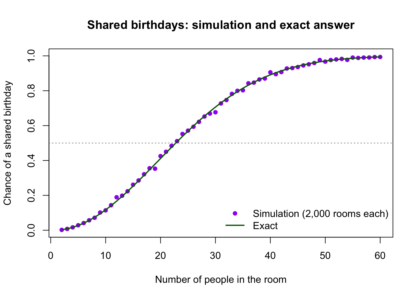
The purple points scatter a little around the green curve, which is what Monte Carlo noise looks like.
In Numerical Methods in Practice, we found the first year a population reached a target with which(). The same idea finds the smallest room where the chance reaches 50%:
sizes[which(exact >= 0.5)[1]][1] 23sizes[which(estimate >= 0.5)[1]][1] 23Only 23 people are needed for better-than-even odds. How large must a room be for a 90% chance? Change 0.5 to 0.9 and find out.
Look back at the shapes from Empirical Models in Practice. This curve rises slowly, then steeply, then levels off near 1, an S-shape. A chance can never go above 1, so a polynomial fit to these points would be a poor choice for predicting larger rooms.
Real birthdays aren’t spread evenly. In the United States, more babies are born in late summer and early fall than in winter. Would that make a shared birthday more likely or less likely than our model says? Think about it before trying it.
sample() accepts a prob argument that makes some values more likely than others. This version makes days 182–273 (roughly July through September) 1.5 times as likely as other days. The 1.5 is a made-up number for exploring the idea, not real birth data.
set.seed(33)
day_weights <- rep(1, 365)
day_weights[182:273] <- 1.5

for (run in 1:runs) {
  birthdays <- sample(1:365, class_size, replace = TRUE, prob = day_weights)
  shared[run] <- any(duplicated(birthdays))
}

mean(shared)
[1] 0.568Compare with the even-birthdays answer for 25 people (about 0.57). Did it go up? Uneven birthdays crowd more people onto the popular days, so matches should become more likely, but with these weights the true increase is only about one percentage point. That’s smaller than the run-to-run spread we saw earlier, so a single run of 2,000 rooms can’t reliably detect it. Try changing 1.5 to 3: the increase becomes large enough to see clearly.
Two lessons here. The exact formula can’t handle uneven birthdays at all, but the simulation needed only one changed line. And a small effect needs many runs before a simulation can tell it apart from noise.