set.seed(201)
x <- seq(0, 4 * pi, by = 0.1)
y <- 2 * sin(x) + runif(length(x), -0.5, 0.5)
wave <- data.frame(x = x, y = y)

plot(wave$x, wave$y, pch = 16, col = "purple",
     xlab = "x", ylab = "y", main = "Noisy wave data")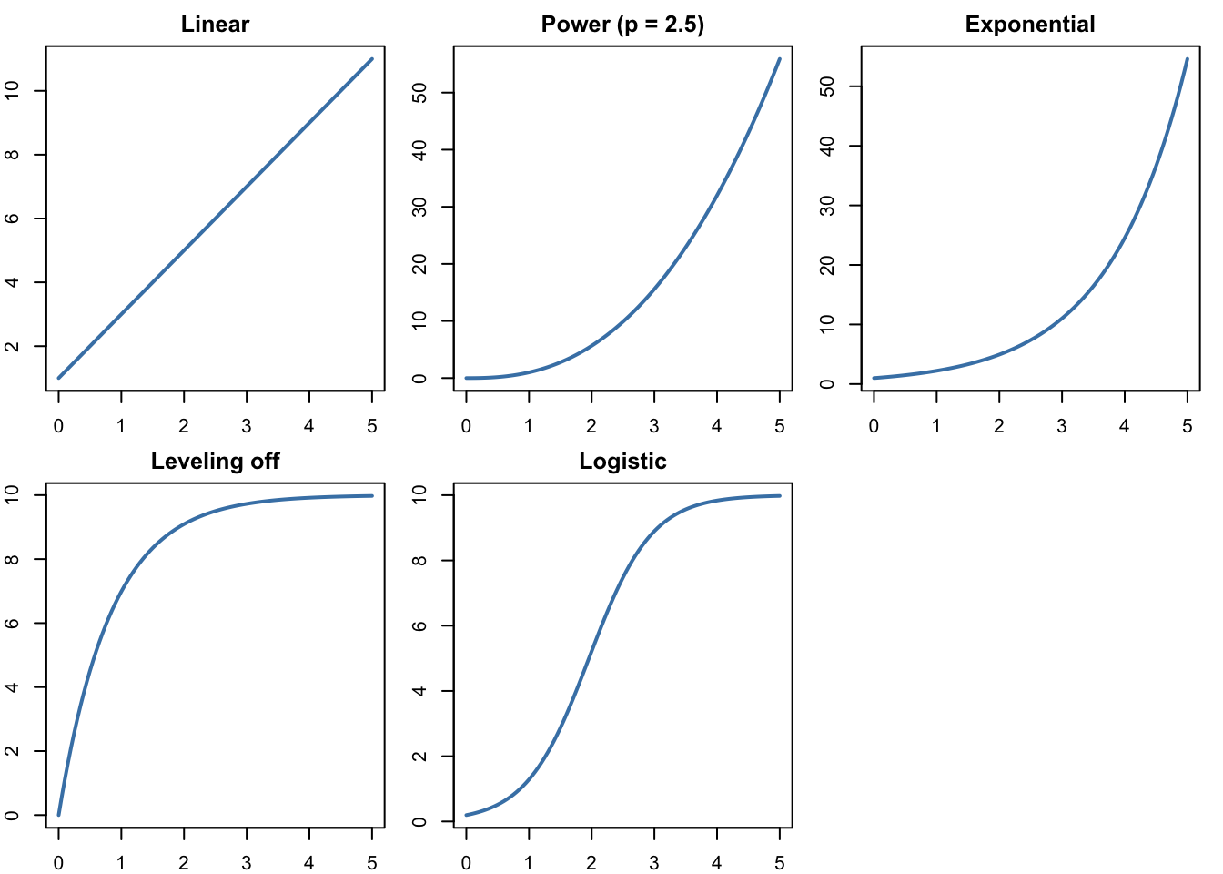
We’ll start with data where we know the right answer, because we make it ourselves. Each \(y\) value is \(2\sin(x)\) plus a little random noise between −0.5 and 0.5, like measurement error. set.seed() makes everyone’s “random” noise the same.
set.seed(201)
x <- seq(0, 4 * pi, by = 0.1)
y <- 2 * sin(x) + runif(length(x), -0.5, 0.5)
wave <- data.frame(x = x, y = y)
plot(wave$x, wave$y, pch = 16, col = "purple",
xlab = "x", ylab = "y", main = "Noisy wave data")
Now pretend we don’t know where the data came from, and fit three models with lm():
lm() treats \(\sin(x)\) as a new column of numbers, just as it treated \(x^2\) on Monday.line_fit <- lm(y ~ x, data = wave)
poly_fit <- lm(y ~ x + I(x^2) + I(x^3) + I(x^4) + I(x^5), data = wave)
sine_fit <- lm(y ~ sin(x), data = wave)
coef(sine_fit)(Intercept) sin(x)
-0.04944213 2.02237513 The sine model found \(y \approx -0.05 + 2.02\sin(x)\), very close to the \(2\sin(x)\) we used to make the data.
To draw each model, make a fine grid of \(x\) values and let predict() compute the model’s \(y\) at each one:
x_grid <- data.frame(x = seq(0, 4 * pi, by = 0.05))

plot(wave$x, wave$y, pch = 16, col = "purple",
     xlab = "x", ylab = "y", main = "Three models for the wave data")
lines(x_grid$x, predict(line_fit, x_grid), col = "firebrick", lwd = 2)
lines(x_grid$x, predict(poly_fit, x_grid), col = "orange", lwd = 2)
lines(x_grid$x, predict(sine_fit, x_grid), col = "darkgreen", lwd = 2)
legend("bottomleft", c("Line", "Degree 5", "Sine"),
       col = c("firebrick", "orange", "darkgreen"), lwd = 2, bty = "n")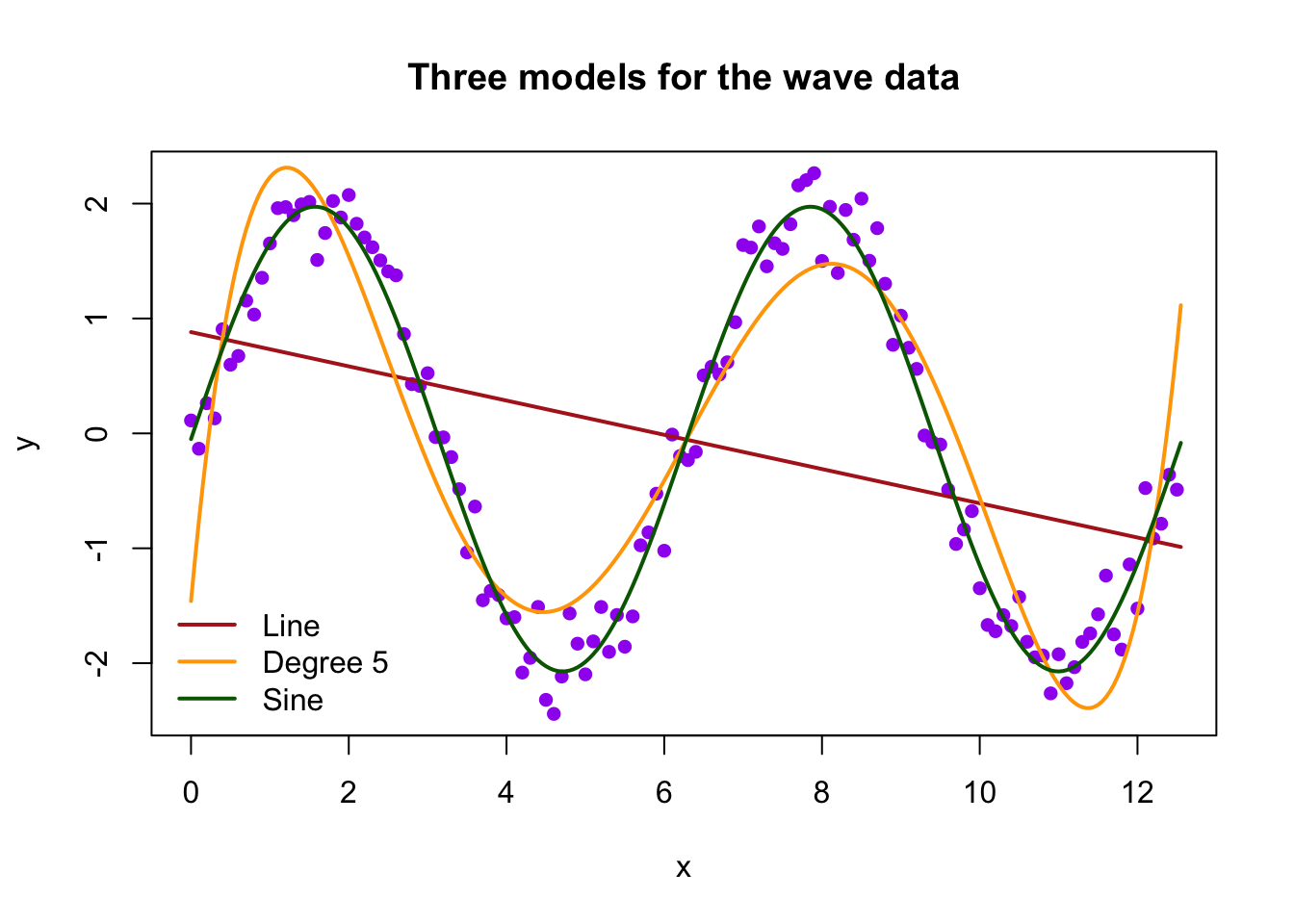
The line is hopeless. The polynomial does a decent job of following the wave, and the sine curve does best. The sums of squared residuals agree:
c(line = sum(resid(line_fit)^2),
  degree_5 = sum(resid(poly_fit)^2),
  sine = sum(resid(sine_fit)^2))
line degree_5 sine
227.520576 35.978248 7.544174 The data run from \(x = 0\) to \(4\pi \approx 12.6\). Let’s predict at two points inside that range and two outside it, and compare with the true value \(2\sin(x)\):
new_x <- data.frame(x = c(5, 11, 16, 20))
data.frame(x = new_x$x,
           true_value = round(2 * sin(new_x$x), 2),
           line = round(predict(line_fit, new_x), 2),
           degree_5 = round(predict(poly_fit, new_x), 2),
           sine = round(predict(sine_fit, new_x), 2))
x true_value line degree_5 sine
1 5 -1.92 0.14 -1.39 -1.99
2 11 -2.00 -0.76 -2.19 -2.07
3 16 -0.58 -1.50 136.05 -0.63
4 20 1.83 -2.10 1080.23 1.80Inside the data, the polynomial is in the right neighborhood. Outside, it predicts 136 at \(x = 16\) and over 1,000 at \(x = 20\), when the true values stay between −2 and 2. A picture shows why:
x_wide <- data.frame(x = seq(0, 20, by = 0.05))

plot(wave$x, wave$y, pch = 16, col = "purple",
     xlim = c(0, 20), ylim = c(-4, 4),
     xlab = "x", ylab = "y", main = "The same models beyond the data")
lines(x_wide$x, predict(poly_fit, x_wide), col = "orange", lwd = 2)
lines(x_wide$x, predict(sine_fit, x_wide), col = "darkgreen", lwd = 2)
abline(v = 4 * pi, lty = 3, col = "gray50")   # end of the data
legend("bottomleft", c("Degree 5", "Sine"), col = c("orange", "darkgreen"),
       lwd = 2, bty = "n")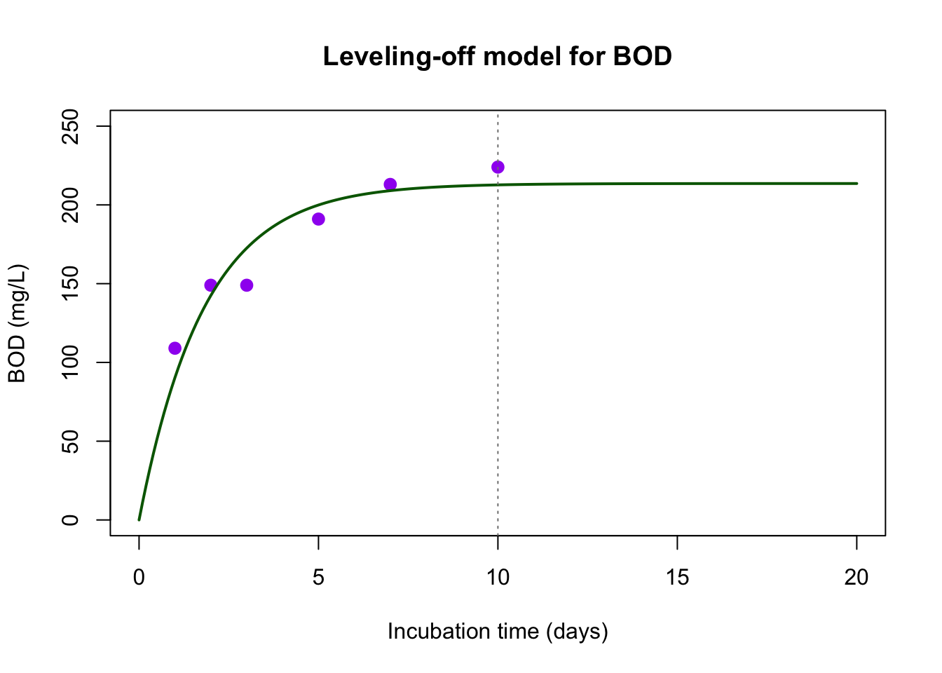
Past the dotted line, the polynomial’s biggest term, \(x^5\), takes over and the curve shoots off the plot. The sine curve keeps waving, because it has the right shape. A polynomial can imitate a wave over a short range, but it isn’t a wave.
Of course, we only knew to try \(\sin(x)\) because we made the data. With real data, the shape has to come from looking at the data and from what we know about the system.
This mystery data set also waves, but it was made a little differently:
set.seed(8)
mystery <- data.frame(x = x, y = 1 + 1.5 * cos(x) + runif(length(x), -0.5, 0.5))
Plot it, fit lm(y ~ sin(x), data = mystery), and draw the fitted curve. What goes wrong? Look at where the data start at \(x = 0\), then try a model with cos(x) instead. Compare the two sums of squared residuals.
sin_try <- lm(y ~ sin(x), data = mystery)
cos_try <- lm(y ~ cos(x), data = mystery)

plot(mystery$x, mystery$y, pch = 16, col = "purple",
     xlab = "x", ylab = "y", main = "Mystery wave data")
lines(x_grid$x, predict(sin_try, x_grid), col = "firebrick", lwd = 2)
lines(x_grid$x, predict(cos_try, x_grid), col = "darkgreen", lwd = 2)
legend("bottomleft", c("Sine", "Cosine"), col = c("firebrick", "darkgreen"),
       lwd = 2, bty = "n")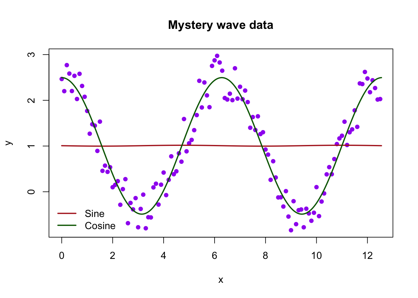
coef(cos_try)(Intercept) cos(x)
1.003412 1.492960 c(sine = sum(resid(sin_try)^2), cosine = sum(resid(cos_try)^2)) sine cosine
150.92154 10.13217 The sine model comes out nearly flat. The data start at a peak, and \(\sin(x)\) starts at 0, so no multiple of \(\sin(x)\) can line up with them. The cosine model finds about \(1.0 + 1.49\cos(x)\), matching how the data were made. Even when the general shape (a wave) is right, the details matter.
Now some real data. Biochemical oxygen demand (BOD) measures how much oxygen bacteria use while breaking down waste in a water sample. These six NIST measurements track BOD over 10 days of incubation.
boxbod <- read.csv("boxbod.csv")
boxbod
days bod
1 1 109
2 2 149
3 3 149
4 5 191
5 7 213
6 10 224With six points, a polynomial of degree 5 has six coefficients, so it can pass through every point exactly. Its residuals are all zero (up to rounding). Compare it with a quadratic, which has just one more term than a line:
quad_bod <- lm(bod ~ days + I(days^2), data = boxbod)
poly5_bod <- lm(bod ~ days + I(days^2) + I(days^3) + I(days^4) + I(days^5),
                data = boxbod)
round(resid(poly5_bod), 6)
1 2 3 4 5 6
0 0 0 0 0 0 day_grid <- data.frame(days = seq(0.5, 11, by = 0.05))
plot(boxbod$days, boxbod$bod, pch = 16, cex = 1.3, col = "purple",
xlim = c(0.5, 11), ylim = c(0, 400),
xlab = "Incubation time (days)", ylab = "BOD (mg/L)",
main = "Two polynomial models for BOD")
lines(day_grid$days, predict(quad_bod, day_grid), col = "steelblue", lwd = 2)
lines(day_grid$days, predict(poly5_bod, day_grid), col = "firebrick", lwd = 2)
legend("topleft", c("Quadratic", "Degree 5"), col = c("steelblue", "firebrick"),
lwd = 2, bty = "n")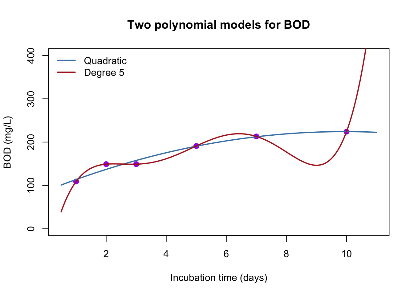
new_days <- data.frame(days = c(8, 12, 20))
data.frame(days = new_days$days,
           quadratic = round(predict(quad_bod, new_days)),
           degree_5 = round(predict(poly5_bod, new_days)))
days quadratic degree_5
1 8 219 177
2 12 218 1577
3 20 83 121395The degree-5 polynomial is “perfect” on the data and absurd everywhere else. It predicts BOD dropping to 177 on day 8 (between measurements of 213 and 224) and over 100,000 on day 20. It has memorized six numbers rather than learning a trend. The quadratic misses the points a bit but behaves sensibly inside the data. Even so, it turns downward by day 20, and BOD can’t decrease: oxygen that bacteria have used doesn’t come back.
Zero residuals aren’t the goal. A model needs a shape that makes sense for the system.
Before fitting anything, look at the data and ask what kind of function could follow it. A few shapes cover most of what we’ll see (the textbook’s Module 8.2 tours them in more detail):
| Shape | Form | What it looks like |
|---|---|---|
| Linear | \(y = b + mx\) | changes by the same amount each step |
| Power | \(y = a x^p\) | curves up (\(p > 1\)) or bends over (\(0 < p < 1\)) |
| Exponential | \(y = a e^{kx}\) | grows by the same fraction each step |
| Leveling off | \(y = a\left(1 - e^{-kx}\right)\) | starts at 0, rises quickly, approaches \(a\) |
| Wave | \(y = b + c\sin(x)\) | repeats; goes up and down forever |
par(mfrow = c(2, 3), mar = c(2, 2, 2, 1))
curve(1 + 2 * x, 0, 5, main = "Linear", lwd = 2, col = "steelblue")
curve(x^2.5, 0, 5, main = "Power (p = 2.5)", lwd = 2, col = "steelblue")
curve(exp(0.8 * x), 0, 5, main = "Exponential", lwd = 2, col = "steelblue")
curve(10 * (1 - exp(-1.2 * x)), 0, 5, main = "Leveling off", lwd = 2,
      col = "steelblue")
curve(2 * sin(3 * x), 0, 5, main = "Wave", lwd = 2, col = "steelblue")
par(mfrow = c(1, 1))
A polynomial can imitate any of these over a short range, which is exactly why it’s dangerous outside that range.
Which of these shapes fits what we know about BOD? Bacteria use oxygen quickly at first, then slow down as their food runs out, and BOD should be 0 at day 0. That’s the leveling-off shape, and it’s the model NIST uses for this data set. Fitting it takes a technique beyond lm(), because \(k\) sits inside the exponential, but choosing the shape is the important step.