EMPTY <- 0
TREE <- 1
BURNING <- 2A model made of cells
Our earlier models tracked a few numbers over time: a population, a temperature, the sizes of S, I, and R. A cellular automaton tracks a whole grid of cells instead. Each cell holds a state, and at every time step, every cell follows the same simple rule.
In the fire model, each cell has one of three states:
| Value | Name | Meaning |
|---|---|---|
| 0 | EMPTY |
bare ground, no tree |
| 1 | TREE |
a tree that isn’t burning |
| 2 | BURNING |
a tree that’s on fire |
Giving the values names makes the code say what it means. forest[i, j] == BURNING is easier to read and check than forest[i, j] == 2.
Build a forest
A grid of numbers in R is a matrix. forest[i, j] is the cell in row i and column j, just as population[i] was one entry of a vector.
Each cell gets a tree with probability prob_tree, the tree density. Before running this: in a 10 × 10 forest with prob_tree = 0.7, about how many trees do you expect?
set.seed(1031)
n <- 10
prob_tree <- 0.7

forest <- matrix(EMPTY, nrow = n, ncol = n)    # start with all bare ground
forest[runif(n * n) < prob_tree] <- TREE       # one random draw per cell
forest
[,1] [,2] [,3] [,4] [,5] [,6] [,7] [,8] [,9] [,10]
[1,] 0 0 0 1 0 1 1 1 1 1
[2,] 1 0 0 1 0 1 1 1 1 1
[3,] 1 1 0 1 0 1 1 1 1 1
[4,] 0 1 0 0 1 1 0 1 1 1
[5,] 1 1 0 0 1 1 1 1 0 1
[6,] 1 1 1 1 1 1 0 1 1 1
[7,] 1 1 1 1 0 1 1 1 0 1
[8,] 1 0 0 0 1 1 1 0 0 1
[9,] 1 0 1 1 1 1 1 1 1 1
[10,] 0 1 1 1 1 1 1 0 0 1sum(forest == TREE)[1] 72runif(n * n) makes 100 draws, one per cell, and every draw below 0.7 turns its cell into a tree. As with mean(outcome == "road") in Project 4, sum(forest == TREE) counts the TRUE values.
A printed matrix is hard to read, so we’ll color each cell by its value. image() draws a matrix, but upside down and sideways from how it prints. The line below flips it so the picture matches the printout. You don’t need to memorize it; copy it whenever you want to see the forest.
forest_colors <- c("wheat", "forestgreen", "orangered")  # EMPTY, TREE, BURNING

image(t(forest[n:1, ]), col = forest_colors, zlim = c(0, 2),
      axes = FALSE, asp = 1, main = "A 10 × 10 forest, density 0.7")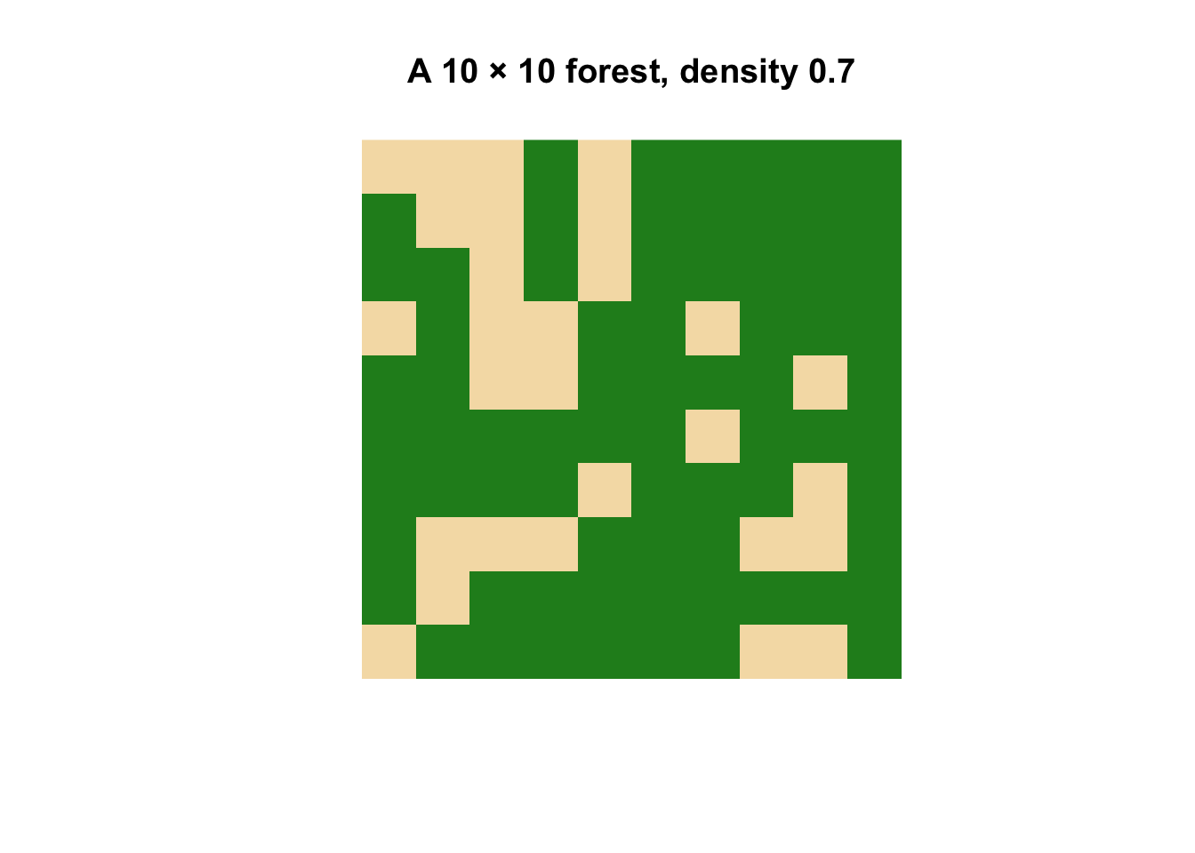
The rule
At each time step, a cell’s next state depends on the cell itself and its four neighbors: the cells directly north, east, south, and west. Diagonal cells don’t count.
- An empty cell stays empty.
- A burning tree burns down and becomes empty.
- A tree with at least one burning neighbor catches fire.
- Any other tree stays a tree.
That’s the whole model. Nothing in the rule mentions the forest as a whole, only one cell and its neighbors.
What about the edges?
A cell in the top row has no neighbor to the north, so forest[i - 1, j] would ask for row 0, which doesn’t exist. We’ll solve that by putting a ring of bare ground around the forest, like a firebreak. Then we update only the inside cells, rows and columns 2 through n + 1, and every one of them has four real neighbors.
Light the fire and take one step
Build a 40 × 40 forest inside a ring of bare ground, and set the center tree on fire:
set.seed(1032)
n <- 40
prob_tree <- 0.7

forest <- matrix(EMPTY, nrow = n + 2, ncol = n + 2)    # includes the ring
inside <- 2:(n + 1)
forest[inside, inside][runif(n * n) < prob_tree] <- TREE
center <- n / 2 + 1
forest[center, center] <- BURNING
Now one time step. Notice that we read neighbors from the old grid, forest, and write the results into a new grid, new_forest. It’s the same reason we saved old before an RK2 update. If we changed forest as we went, a tree that caught fire a moment ago could spread fire again in the same step.
new_forest <- forest

for (i in inside) {
  for (j in inside) {
    if (forest[i, j] == BURNING) {
      new_forest[i, j] <- EMPTY                 # burns down
    } else if (forest[i, j] == TREE) {
      if (forest[i - 1, j] == BURNING || forest[i, j + 1] == BURNING ||
          forest[i + 1, j] == BURNING || forest[i, j - 1] == BURNING) {
        new_forest[i, j] <- BURNING             # catches fire
      }
    }
  }
}

forest <- new_forest
sum(forest == BURNING)
[1] 2|| means “or”: the tree catches fire if the north or east or south or west neighbor is burning. How many trees are burning after one step? Can you explain why it’s at most 4?
Many steps
To run the fire, put the step inside a time loop. We’ll draw the forest at a few times to watch the fire move. par(mfrow = c(2, 3)) puts six graphs on one page, two rows of three.
set.seed(1032)
forest <- matrix(EMPTY, nrow = n + 2, ncol = n + 2)
forest[inside, inside][runif(n * n) < prob_tree] <- TREE
forest[center, center] <- BURNING

par(mfrow = c(2, 3), mar = c(1, 1, 2, 1))

for (t in 0:30) {
  if (t %in% c(0, 4, 8, 12, 20, 30)) {
    image(t(forest[(n + 2):1, ]), col = forest_colors, zlim = c(0, 2),
          axes = FALSE, asp = 1, main = paste("t =", t))
  }
  new_forest <- forest
  for (i in inside) {
    for (j in inside) {
      if (forest[i, j] == BURNING) {
        new_forest[i, j] <- EMPTY
      } else if (forest[i, j] == TREE) {
        if (forest[i - 1, j] == BURNING || forest[i, j + 1] == BURNING ||
            forest[i + 1, j] == BURNING || forest[i, j - 1] == BURNING) {
          new_forest[i, j] <- BURNING
        }
      }
    }
  }
  forest <- new_forest
}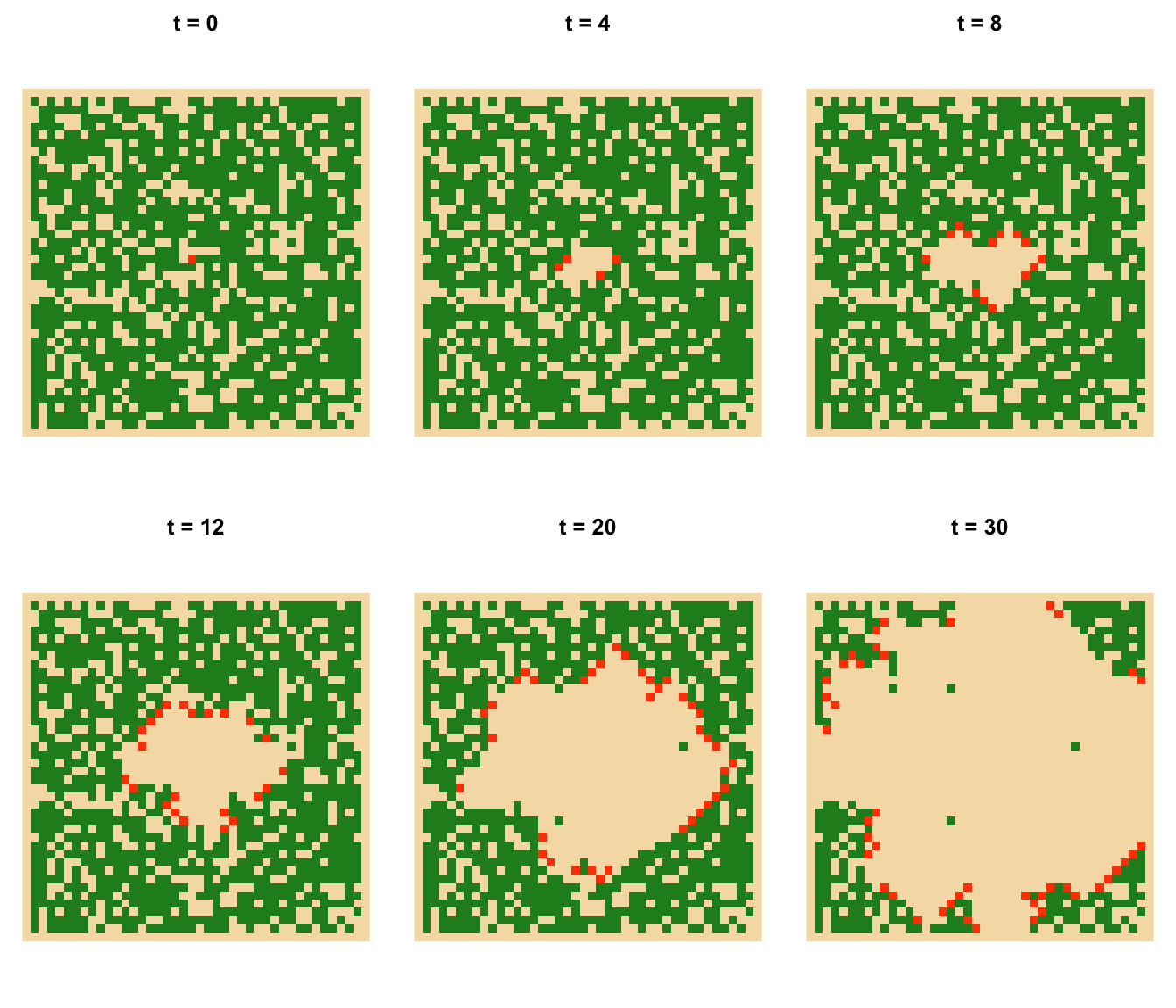
par(mfrow = c(1, 1))The fire moves outward as a ragged front and leaves bare ground behind it. Some trees survive because no burning neighbor ever touched them. A diagonal neighbor isn’t enough.
Now change prob_tree to 0.5 and run it again. What happens?
Ask a question one forest can’t answer
How does tree density change the fraction of trees that burn? One forest is one example, just like one hike in Project 4. We need many forests at each density, the same Monte Carlo idea we’ve used for two weeks.
This code doesn’t introduce any new ideas, but it nests the loops deeply, so read it from the inside out:
- The innermost loops are the step we just wrote.
while (any(forest == BURNING))keeps stepping as long as any tree is still burning. A fire always burns out, because nothing regrows, so the loop always ends.- The
runloop builds and burns 20 forests at one density and records the fraction of trees that burned in each. - The outer loop moves through the densities.
Before running it: sketch the curve you expect for the fraction burned against tree density, from 0.3 to 0.9. A straight line? Something else?
set.seed(1033)
n <- 30
inside <- 2:(n + 1)
center <- n / 2 + 1
densities <- seq(0.3, 0.9, by = 0.05)
runs <- 20
mean_burned <- numeric(length(densities))

for (k in seq_along(densities)) {
  burned <- numeric(runs)
  for (run in 1:runs) {
    forest <- matrix(EMPTY, nrow = n + 2, ncol = n + 2)
    forest[inside, inside][runif(n * n) < densities[k]] <- TREE
    forest[center, center] <- BURNING
    trees_at_start <- sum(forest != EMPTY)

    while (any(forest == BURNING)) {
      new_forest <- forest
      for (i in inside) {
        for (j in inside) {
          if (forest[i, j] == BURNING) {
            new_forest[i, j] <- EMPTY
          } else if (forest[i, j] == TREE) {
            if (forest[i - 1, j] == BURNING || forest[i, j + 1] == BURNING ||
                forest[i + 1, j] == BURNING || forest[i, j - 1] == BURNING) {
              new_forest[i, j] <- BURNING
            }
          }
        }
      }
      forest <- new_forest
    }

    burned[run] <- (trees_at_start - sum(forest == TREE)) / trees_at_start
  }
  mean_burned[k] <- mean(burned)
}

data.frame(density = densities, mean_fraction_burned = round(mean_burned, 2))
density mean_fraction_burned
1 0.30 0.02
2 0.35 0.02
3 0.40 0.03
4 0.45 0.06
5 0.50 0.09
6 0.55 0.23
7 0.60 0.48
8 0.65 0.79
9 0.70 0.95
10 0.75 0.99
11 0.80 1.00
12 0.85 1.00
13 0.90 1.00plot(densities, mean_burned, type = "o", pch = 16, col = "orangered",
ylim = c(0, 1), xlab = "Tree density (prob_tree)",
ylab = "Mean fraction of trees burned",
main = "One fire in a 30 × 30 forest (20 forests per density)")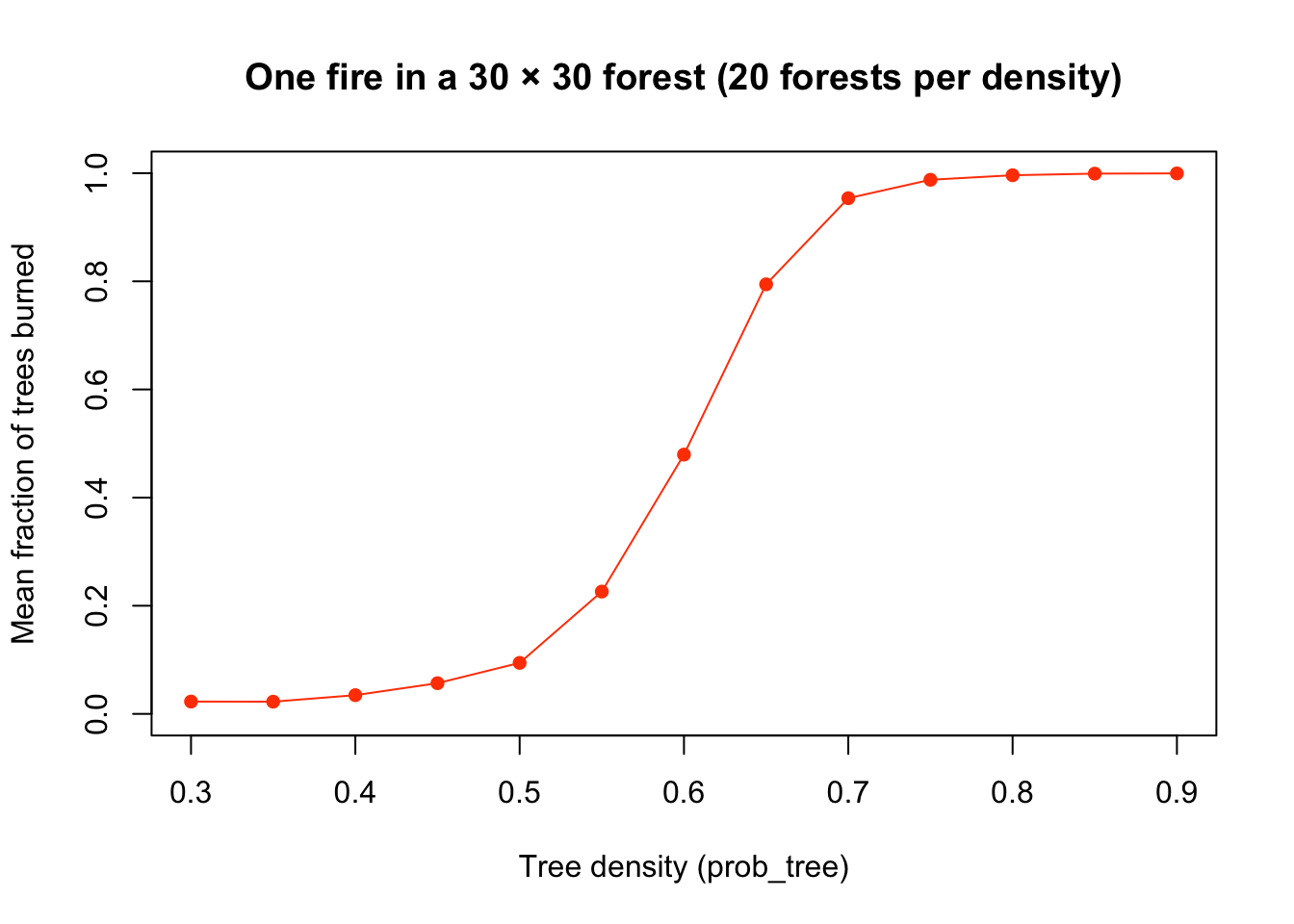
The curve isn’t a straight line. At low densities, the fire almost always dies out near where it started. At high densities, it sweeps nearly the whole forest. In between, a small change in density makes a big change in the outcome. That’s a tipping point (physicists call it a percolation threshold), and it comes from nothing more than each tree checking four neighbors.
Look back at the guesses you made at the start. How close were they?
Near the tipping point, would 20 forests be enough? Why might the results vary the most there?
If we have time: wet wood
The book’s model gives each tree a chance to resist catching fire, which it calls immunity. To try it, set prob_immune <- 0.25 and replace the “catches fire” line with this, so a burning neighbor sets a tree on fire only 75% of the time:
if (runif(1) >= prob_immune) {
  new_forest[i, j] <- BURNING
}
Does the tipping point move to a higher or lower density? Why?
How the book’s model differs
Our model keeps the key idea and drops three details from the book’s version (pp. 438–439):
- Edges. The book wraps the grid around, so the top row’s north neighbor is the bottom row, like a forest drawn on a donut. We used a firebreak ring instead.
- Immunity. The book lets a tree resist catching fire. That’s the “if we have time” change above.
- Lightning. The book lets a tree with no burning neighbors catch fire with a small probability, so new fires can start anywhere.