Module 9.2 · Random inputs, repeated experiments, and an estimate of π
TipToday’s question
Can we estimate the area of a circle by throwing virtual darts? Each throw is unpredictable, but the fraction of hits becomes useful when we throw many darts.
NoteReading
Read textbook Module 9.2, “Simulations.” Its dartboard example estimates an area by counting random hits. Our comparison of uniform and normal random numbers is a first look at Module 9.3, “Random Numbers from Various Distributions”; we are not covering all of 9.3 today. Download the complete R script after coding along.
What changes when a model uses chance?
Our earlier population models gave the same answer every time we ran the same code with the same parameters. A stochastic model includes chance, so repeated runs can give different answers. A Monte Carlo simulation uses random draws to estimate a quantity or explore possible outcomes.
Before coding, discuss: if two correct simulations use the same assumptions but report slightly different estimates, has one of them necessarily made an error?
Computers generate pseudorandom numbers: an algorithm produces a sequence that behaves like random draws for our purposes. We can set a seed to reproduce the sequence while debugging or comparing code. A seed does not make the model deterministic in the real-world sense; it just lets us replay the same draws.
Where do random numbers come from?
For our simulations, replaying the same draws with set.seed() is useful: we can check our code and compare changes fairly. For security, however, an attacker must not be able to predict the seed. These links show two ways to obtain unpredictable input from the physical world:
Read: How Cloudflare uses lava lamps. Images of the lamps contribute randomness to a cryptographic generator; Cloudflare combines this with other sources. The lamps are not simply a replacement for set.seed() in R.
Explore: RANDOM.ORG. It offers random numbers derived from atmospheric noise, including integer and Gaussian generators.
Which goal matters more for our code-along: reproducing a run or keeping its numbers unpredictable to someone else? Why might a security application answer differently?
Two ways to draw random numbers in R
runif() draws from a uniform distribution: equal-length parts of the specified interval have equal chances. rnorm() draws from a normal distribution: values near the mean are more common, and values far from it are possible but less common.
Predict before running this: do the second and third lines mean the same thing?
set.seed(201) # reproduce these draws when we rerun the pagerunif(5, min =0, max =1) # five values spread uniformly from 0 to 1
The first argument is how many values to draw. For runif(), min and max set the interval. For rnorm(), mean locates the center and sd controls the spread. In particular, sd is not a minimum or maximum; a normal distribution has no hard cutoff.
See the shapes
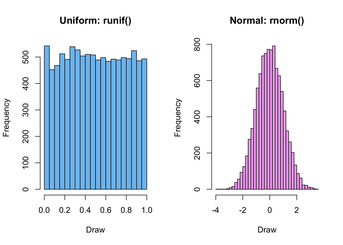
Five draws are not enough to reveal a distribution. Draw many values and compare two histograms. What is different about their shapes? What would happen to the second histogram if we doubled sd?
uniform_draws <-runif(10000, min =0, max =1)normal_draws <-rnorm(10000, mean =0, sd =1)par(mfrow =c(1, 2))hist(uniform_draws, breaks =20, col ="skyblue2",main ="Uniform: runif()", xlab ="Draw")hist(normal_draws, breaks =30, col ="plum2",main ="Normal: rnorm()", xlab ="Draw")
par(mfrow =c(1, 1))
Neither distribution is automatically “more realistic.” We choose a distribution by asking what kinds of values are possible and how likely each range should be. For example, a random location in a square calls for uniform coordinates. A measured quantity that clusters around a typical value might call for a normal model, if the data support it.
A Monte Carlo dartboard
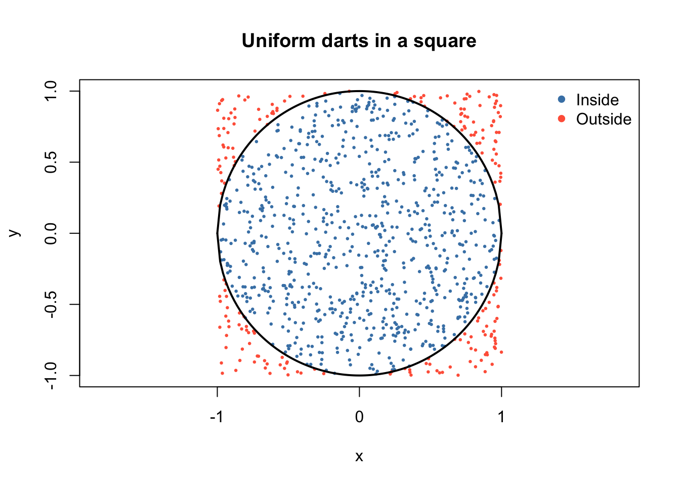
Imagine a circle of radius 1 inside a square that runs from \(-1\) to \(1\) on both axes. The square has area \(2\times2=4\). The circle has area \(\pi(1)^2=\pi\). If darts land uniformly throughout the square, the fraction inside the circle should be close to \(\pi/4\) when we throw many darts:
\[
\pi \approx 4\frac{\text{number of darts inside the circle}}{\text{total number of darts}}.
\]
A dart at \((x,y)\) is inside or on the circle when \(x^2+y^2\leq1\). Which of these hits: \((0.5,0.5)\) or \((0.9,0.9)\)? Check without plotting first.
One dart before one thousand
x_one <-runif(1, min =-1, max =1)y_one <-runif(1, min =-1, max =1)x_one^2+ y_one^2<=1
[1] FALSE
Now repeat that test in a loop. Start by changing number_of_darts to 10 and looking at the results. Then return it to 1000 for the rest of the page. Keep the set.seed() call so a fresh render reproduces the same example.
set.seed(201)number_of_darts <-1000x <-numeric(number_of_darts)y <-numeric(number_of_darts)inside <-logical(number_of_darts)for (i in1:number_of_darts) { x[i] <-runif(1, min =-1, max =1) y[i] <-runif(1, min =-1, max =1) inside[i] <- x[i]^2+ y[i]^2<=1}number_inside <-sum(inside) # TRUE counts as 1; FALSE counts as 0pi_estimate <-4* number_inside / number_of_dartsdata.frame(darts = number_of_darts,hits = number_inside,estimate = pi_estimate,absolute_error =abs(pi_estimate - pi))
Why multiply the hit fraction by 4? Does the result have to be below the true value of \(\pi\)? What would be a suspicious result—for example, could this calculation ever return 5?
Show the simulated experiment
plot(x, y, pch =16, cex =0.45,col =ifelse(inside, "steelblue", "tomato"),xlim =c(-1, 1), ylim =c(-1, 1), asp =1,xlab ="x", ylab ="y", main ="Uniform darts in a square")curve(sqrt(1- x^2), from =-1, to =1, add =TRUE, lwd =2)curve(-sqrt(1- x^2), from =-1, to =1, add =TRUE, lwd =2)legend("topright", c("Inside", "Outside"),col =c("steelblue", "tomato"), pch =16, bty ="n")
Experiment with the number of darts
Rerun the simulation and plot with 10, 100, 1000, and 10000 darts. Record what you notice. Remove or change set.seed(201)only after you have compared the different sizes; otherwise two changes happen at once.
Darts
Estimate of \(\pi\)
Absolute error
What does the plot look like?
10
100
1000
10000
More darts tend to make the estimate more reliable, but a single larger run is not guaranteed to be closer than a particular smaller run. Try running 1000 darts twice without resetting the seed. Did the answers match? What stayed the same about the model, and what changed?
ImportantThe distribution is part of the model
Our area argument works because the darts are uniformly located in the square. Replacing the coordinates with rnorm() would crowd darts near the center (and allow coordinates outside the square). Then “fraction inside × 4” would no longer estimate the circle’s area. A simulation can run perfectly and still answer the wrong question if we choose the wrong distribution.
If we have time: compare whole simulations
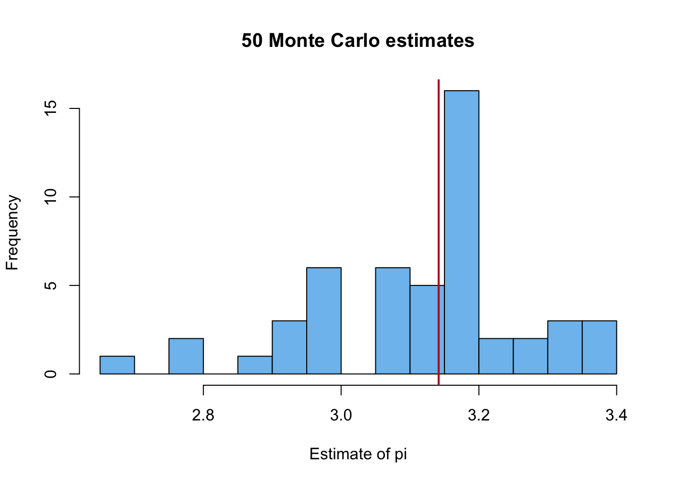
One estimate can be lucky or unlucky. This optional chunk runs 50 independent simulations of 100 darts each. It uses the same circle test but draws each run’s coordinates as vectors. The outer loop stores one estimate per simulation.
set.seed(202)number_of_runs <-50darts_per_run <-100estimates <-numeric(number_of_runs)for (run in1:number_of_runs) { x_run <-runif(darts_per_run, min =-1, max =1) y_run <-runif(darts_per_run, min =-1, max =1) hits_run <- x_run^2+ y_run^2<=1 estimates[run] <-4*sum(hits_run) / darts_per_run}hist(estimates, breaks =12, col ="skyblue2",main ="50 Monte Carlo estimates", xlab ="Estimate of pi")abline(v = pi, col ="firebrick", lwd =2)
How much do individual answers vary? Is the average of the 50 estimates close to \(\pi\)? A simulation result should usually be reported with some sense of variation, not as if one run were an exact answer.