On Monday, a polynomial fit six points perfectly and still made absurd predictions. Today we ask: how do we choose a better model, and how can we test it before trusting its predictions?
NoteReading and code
This is practice with textbook Module 8.3, “Empirical Models,” continuing Monday’s page. Save boxbod.csv in the same folder as your script. The second dataset, pressure, is built into R. Download the complete R script after coding along.
Start with the shape
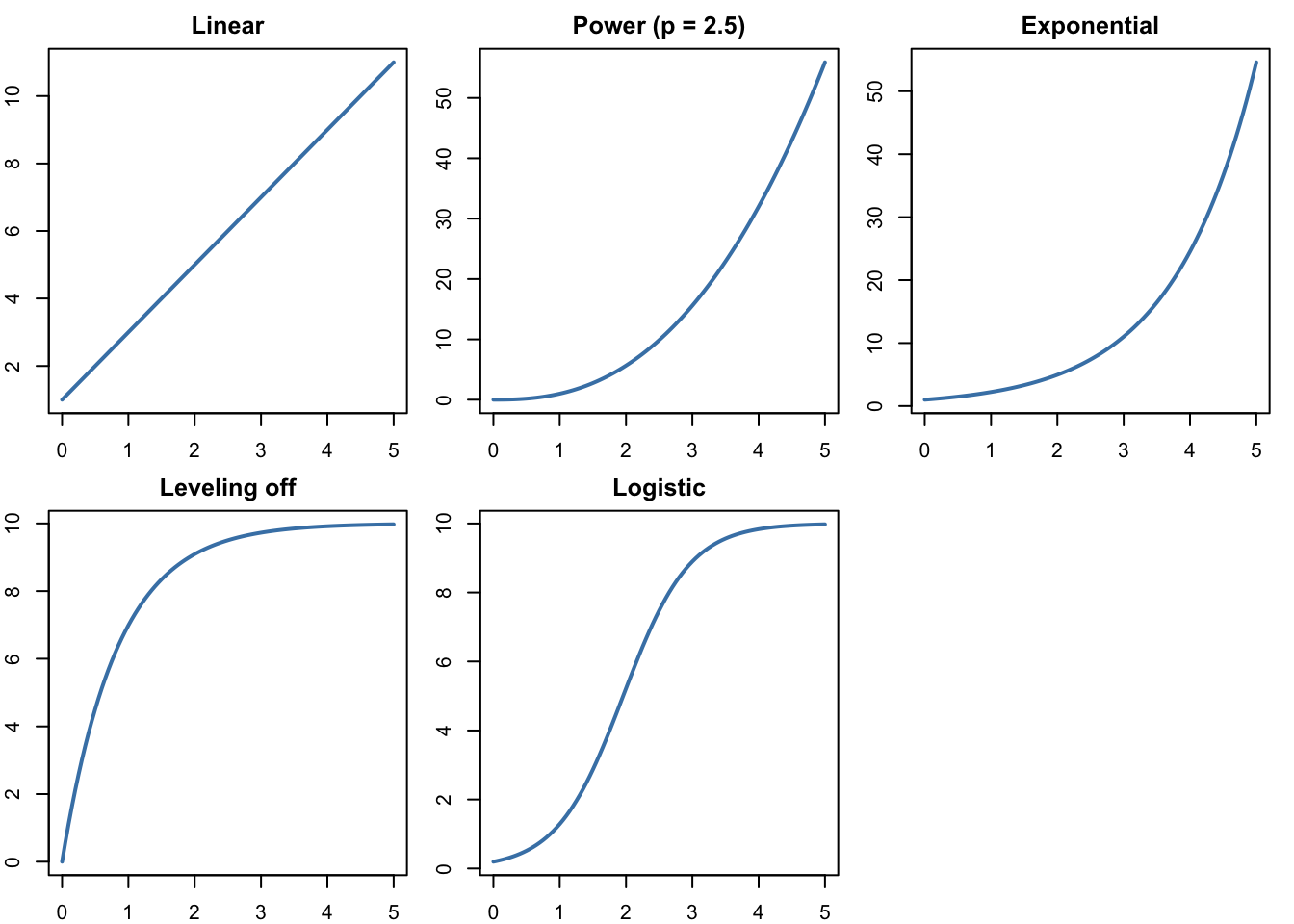
Before fitting anything, look at the data and ask what kind of function could follow it. A few shapes cover most of what we’ll see (the textbook’s Module 8.2 tours them in more detail):
Shape
Form
What it looks like
Linear
\(y = b + mx\)
changes by the same amount each step
Power
\(y = a x^p\)
curves up (\(p > 1\)) or bends over (\(0 < p < 1\))
Exponential
\(y = a e^{kx}\)
grows by the same fraction each step; \(\ln y\) is linear in \(x\)
Leveling off
\(y = a\left(1 - e^{-kx}\right)\)
starts at 0, rises quickly, approaches \(a\)
Logistic
\(y = \dfrac{K}{1 + c e^{-rx}}\)
S-shaped; the solution of constrained growth
par(mfrow =c(2, 3), mar =c(2, 2, 2, 1))curve(1+2* x, 0, 5, main ="Linear", lwd =2, col ="steelblue")curve(x^2.5, 0, 5, main ="Power (p = 2.5)", lwd =2, col ="steelblue")curve(exp(0.8* x), 0, 5, main ="Exponential", lwd =2, col ="steelblue")curve(10* (1-exp(-1.2* x)), 0, 5, main ="Leveling off", lwd =2,col ="steelblue")curve(10/ (1+50*exp(-2* x)), 0, 5, main ="Logistic", lwd =2,col ="steelblue")par(mfrow =c(1, 1))
The shape should come from the data and from what we know about the system. A polynomial can imitate any of these over a short range, which is exactly why it’s dangerous outside that range.
Finish the BOD problem
Recall Monday’s BOD data: oxygen demand rises over 10 days of incubation. Bacteria use oxygen quickly at first, then slow down as their food runs out, and BOD should be 0 at day 0. That’s the leveling-off shape:
\[
\text{BOD} = a\left(1 - e^{-k t}\right),
\]
where \(a\) is the eventual BOD and \(k\) controls how fast it gets there.
boxbod <-read.csv("boxbod.csv")boxbod
  days bod
1    1 109
2    2 149
3    3 149
4    5 191
5    7 213
6   10 224
lm() can’t fit \(k\) directly, because \(k\) sits inside the exponential. But if we pick a value of \(k\), the model is just \(a\) times a known quantity \(z = 1 - e^{-kt}\), and lm() can find the best \(a\). The 0 + in the formula means “no intercept,” because the model has none.
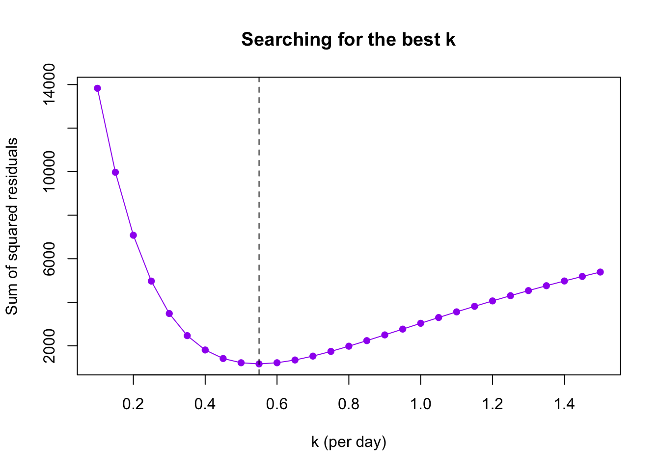
So we use the same strategy as Monday’s power search: try many values of \(k\), and keep the one with the smallest sum of squared residuals.
rates <-seq(0.1, 1.5, by =0.05)ssr <-numeric(length(rates))for (i inseq_along(rates)) { z <-1-exp(-rates[i] * boxbod$days) fit <-lm(boxbod$bod ~0+ z) ssr[i] <-sum(resid(fit)^2)}best_k <- rates[which.min(ssr)]best_k
[1] 0.55
plot(rates, ssr, type ="o", pch =16, col ="purple",xlab ="k (per day)", ylab ="Sum of squared residuals",main ="Searching for the best k")abline(v = best_k, lty =2)
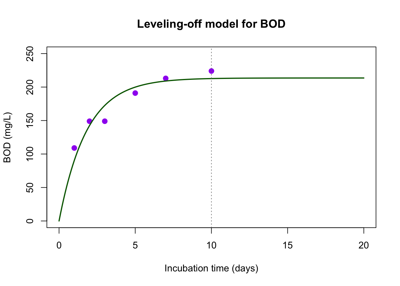
So the model is about \(\text{BOD} = 213.6\left(1 - e^{-0.55t}\right)\). Plot it with the data, and compare its predictions with Monday’s degree-5 polynomial (which predicted 177 at day 8 and over 100,000 at day 20):
day_grid <-seq(0, 20, by =0.1)plot(boxbod$days, boxbod$bod, pch =16, cex =1.3, col ="purple",xlim =c(0, 20), ylim =c(0, 250),xlab ="Incubation time (days)", ylab ="BOD (mg/L)",main ="Leveling-off model for BOD")lines(day_grid, best_a * (1-exp(-best_k * day_grid)), col ="darkgreen", lwd =2)abline(v =10, lty =3, col ="gray50") # last measurement
It misses some points by up to about 20 mg/L (six noisy measurements), but every prediction is believable, even past day 10 (the dotted line), because the shape matches what the bacteria are doing. It’s still a prediction beyond the data, so we’d want a day-20 measurement before relying on it.
R can search for both at once
Our loop only searched \(k\) in steps of 0.05. R’s nls() (“nonlinear least squares”) searches \(a\) and \(k\) together. It needs a starting guess, and ours is a good one:
nls(bod ~ a * (1-exp(-k * days)), data = boxbod,start =list(a =200, k =0.5))
Nonlinear regression model
  model: bod ~ a * (1 - exp(-k * days))
   data: boxbod
       a        k
213.8095   0.5472
 residual sum-of-squares: 1168

Number of iterations to convergence: 7
Achieved convergence tolerance: 2.976e-06
NIST’s certified answer for this dataset is \(a = 213.81\), \(k = 0.5472\). Our grid search came close; nls() matches it.
Fit, then test
A model that fits the data it was built from has passed an easy test. A harder test: hide some data, fit the model to the rest, and see how well it predicts what we hid. This is called validation.
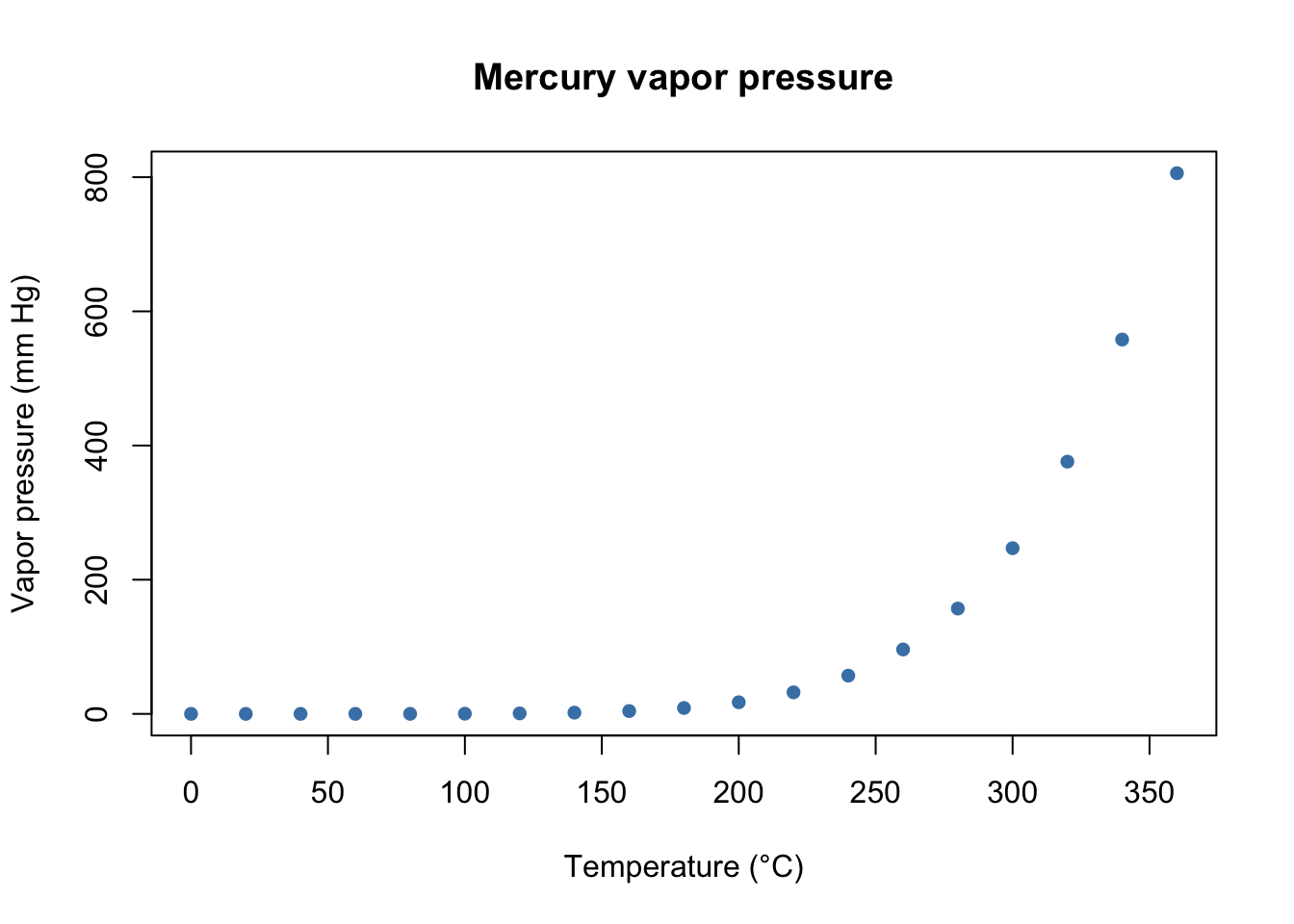
R’s built-in pressure dataset records the vapor pressure of mercury (in millimeters of mercury) at temperatures from 0 to 360 °C:
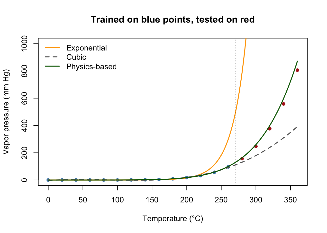
We’ll fit models only to temperatures up to 260 °C (the training data), then predict 280–360 °C (the test data) and compare with the real measurements.
Exponential. The pressure looks exponential, so fit a line to \(\ln(\text{pressure})\) vs. temperature.
Cubic polynomial. Let a flexible curve follow the training data.
Physics-based. Chemistry’s Clausius–Clapeyron relation says \(\ln(\text{pressure})\) is roughly linear in \(1/T\), where \(T\) is the temperature in kelvins.
All three are linear combinations, so lm() fits them all:
expo_fit <-lm(log(pressure) ~ temperature, data = train)cubic_fit <-lm(pressure ~ temperature +I(temperature^2) +I(temperature^3),data = train)physics_fit <-lm(log(pressure) ~I(1/ kelvin), data = train)
For the two log models, predict() returns \(\ln(\text{pressure})\), so we undo the log with exp():
temp_grid <-seq(0, 360, by =2)grid <-data.frame(temperature = temp_grid, kelvin = temp_grid +273.15)plot(pressure$temperature, pressure$pressure, pch =16,col =ifelse(pressure$temperature <=260, "steelblue", "firebrick"),ylim =c(0, 1000), xlab ="Temperature (°C)",ylab ="Vapor pressure (mm Hg)", main ="Trained on blue points, tested on red")lines(temp_grid, exp(predict(expo_fit, grid)), col ="orange", lwd =2)lines(temp_grid, predict(cubic_fit, grid), col ="gray40", lwd =2, lty =2)lines(temp_grid, exp(predict(physics_fit, grid)), col ="darkgreen", lwd =2)abline(v =270, lty =3)legend("topleft", c("Exponential", "Cubic", "Physics-based"),col =c("orange", "gray40", "darkgreen"), lwd =2, lty =c(1, 2, 1),bty ="n")
The cubic and physics-based curves both follow the blue training points closely; the exponential already drifts above the last few. On the red test points they split apart:
The exponential model overshoots wildly: about 38,000 at 360 °C instead of 806.
The cubic falls further and further behind, reaching only about half the real pressure at 360 °C.
The physics-based model stays within about 10% of every test point.
Which one would you trust at 380 °C? Notice that the cubic and physics-based models looked equally good on the training data. Only data the models hadn’t seen could tell them apart.
Here the test points were all at the high end, which is the hardest kind of test (extrapolation). Another common approach is to hide a random sample of points instead. Try it: use sample() to pick 5 rows for the test set, refit, and compare.
If we have time: fit the error of our own methods
Empirical models can describe simulations too. Module 6.4 claimed that the error of Euler, RK2, and RK4 shrinks like \(\Delta t\), \(\Delta t^2\), and \(\Delta t^4\). Let’s measure that (the book’s Module 8.3, Project 10).
The model is \(dP/dt = 0.1P\) with \(P(0) = 100\), run to \(t = 100\). We know the exact answer, \(100e^{10}\), so we can compute the relative error for each method and time step.
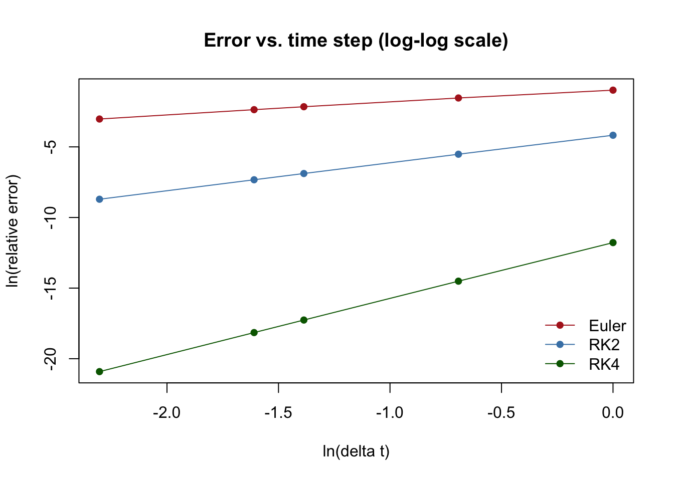
If \(\text{error} = c\,\Delta t^{\,p}\), then taking logs gives \(\ln(\text{error}) = \ln c + p \ln \Delta t\): a line, whose slope is the power \(p\). So fit a line on the log–log scale:
for (m in methods) { slope <-coef(lm(log(errors[, m]) ~log(steps)))[2]cat(m, "error shrinks like delta_t to the power", round(slope, 2), "\n")}
Euler error shrinks like delta_t to the power 0.89
RK2 error shrinks like delta_t to the power 1.97
RK4 error shrinks like delta_t to the power 3.97
plot(log(steps), log(errors[, "Euler"]), type ="o", pch =16, col ="firebrick",ylim =range(log(errors)), xlab ="ln(delta t)", ylab ="ln(relative error)",main ="Error vs. time step (log-log scale)")lines(log(steps), log(errors[, "RK2"]), type ="o", pch =16, col ="steelblue")lines(log(steps), log(errors[, "RK4"]), type ="o", pch =16, col ="darkgreen")legend("bottomright", methods, col =c("firebrick", "steelblue", "darkgreen"),pch =16, lwd =1, bty ="n")
The slopes come out close to 1, 2, and 4. Euler’s is a bit below 1 because \(\Delta t = 1\) is big enough that the pattern hasn’t fully settled in. Our data back up the claim from Module 6.4.
ImportantA workflow for empirical models
Look first. Plot the data and decide what shape is plausible, using what you know about the system.
Fit. Use lm() for linear combinations; transform or search for parameters that sit inside a function.
Check the fit. Plot the model on the original data and look at the residuals.
Test. Predict data the model hasn’t seen. A model that only fits its training data hasn’t earned trust yet.
Respect the range. Every prediction outside the data is a guess, even from a good model.