Numerical Methods in Practice

Today’s question

Suppose a recovering population grows toward a carrying capacity. When will it first reach 500? Will Euler, RK2, and RK4 give the same answer if we take one-year steps?

Reading and code

This is practice with textbook Modules 6.2–6.4, not a new book module. Download the complete R script after coding along. Project 3 asks for Euler and RK2 on a different model; RK4 is not required there.

Return to constrained growth

We will reuse the logistic model from Module 2.3, but pay attention to the numerical method rather than inventing a new model:

\[ \frac{dP}{dt}=rP\left(1-\frac{P}{K}\right). \]

Start with \(P(0)=100\), growth fraction \(r=0.8\) per year, and carrying capacity \(K=1000\). Simulate through year 8. Each method must use these same assumptions; only the update rule will change. We will use a one-year time step first.

Before coding, predict: will the three methods give the same year for reaching 500? How might a large time step affect that answer?

One old population, three ways to step

At the start, the rate is \(0.8(100)(1-100/1000)=72\) population units per year. With \(\Delta t=1\) year:

Euler: use that starting rate for the whole step, giving \(100+72=172\).
RK2: use Euler’s trial value of 172 to get a second rate, then average the starting and trial-end rates. What value do you expect—below or above 172?
RK4: take four trial rates from the same starting value and combine them with weights \(1,2,2,1\). None of its trial values becomes the stored population until the final update.

The population increases faster as it moves away from 100, so Euler’s first step should be the lowest of the three. But that observation does not prove the methods will preserve the same ordering forever; the rate slows again as \(P\) approaches \(K\).

Code all three methods side by side

Keep a separate population vector for each method. At every iteration, read that method’s old value before calculating its trial rates. We do not need to put the simulation inside a function.

start_time <- 0
end_time <- 8
delta_t <- 1                 # years per step
time <- seq(start_time, end_time, by = delta_t)

initial_population <- 100
growth_fraction <- 0.8       # per year
capacity <- 1000
target <- 500

euler <- numeric(length(time))
rk2 <- numeric(length(time))
rk4 <- numeric(length(time))
euler[1] <- initial_population
rk2[1] <- initial_population
rk4[1] <- initial_population

for (i in 2:length(time)) {
  # Euler: one rate at the old population.
  old_euler <- euler[i - 1]
  euler_rate <- growth_fraction * old_euler *
    (1 - old_euler / capacity)
  euler[i] <- old_euler + euler_rate * delta_t

  # RK2: predict an endpoint, then average the old and trial-end rates.
  old_rk2 <- rk2[i - 1]
  rate_1 <- growth_fraction * old_rk2 *
    (1 - old_rk2 / capacity)
  predicted <- old_rk2 + rate_1 * delta_t
  rate_2 <- growth_fraction * predicted *
    (1 - predicted / capacity)
  rk2[i] <- old_rk2 + (rate_1 + rate_2) / 2 * delta_t

  # RK4: four full-step trial changes, all built from the old value.
  old_rk4 <- rk4[i - 1]
  change_1 <- growth_fraction * old_rk4 *
    (1 - old_rk4 / capacity) * delta_t

  trial_mid_1 <- old_rk4 + change_1 / 2
  change_2 <- growth_fraction * trial_mid_1 *
    (1 - trial_mid_1 / capacity) * delta_t

  trial_mid_2 <- old_rk4 + change_2 / 2
  change_3 <- growth_fraction * trial_mid_2 *
    (1 - trial_mid_2 / capacity) * delta_t

  trial_end <- old_rk4 + change_3
  change_4 <- growth_fraction * trial_end *
    (1 - trial_end / capacity) * delta_t

  rk4[i] <- old_rk4 +
    (change_1 + 2 * change_2 + 2 * change_3 + change_4) / 6
}

results <- data.frame(time, euler, rk2, rk4)
round(results[1:4, ], 3)

  time   euler     rk2     rk4
1    0 100.000 100.000 100.000
2    1 172.000 192.966 198.131
3    2 285.933 341.943 354.688
4    3 449.273 531.758 550.152

The first row is the initial population. The next row should be approximately 172.000 (Euler), 192.966 (RK2), and 198.131 (RK4). If your values differ, inspect the first step before looking at the whole eight-year simulation. In particular, all four RK4 trial changes must begin from old_rk4.

Ask the decision question

Find the first recorded time at which each method reaches or exceeds 500. A position in an R vector is not a year, so look up the corresponding value of time.

first_euler <- which(euler >= target)[1]
first_rk2 <- which(rk2 >= target)[1]
first_rk4 <- which(rk4 >= target)[1]

data.frame(
  method = c("Euler", "RK2", "RK4"),
  first_recorded_year = c(time[first_euler],
                          time[first_rk2],
                          time[first_rk4]),
  population_at_that_year = round(c(euler[first_euler],
                                    rk2[first_rk2],
                                    rk4[first_rk4]), 2)
)

  method first_recorded_year population_at_that_year
1  Euler                   4                  647.21
2    RK2                   3                  531.76
3    RK4                   3                  550.15

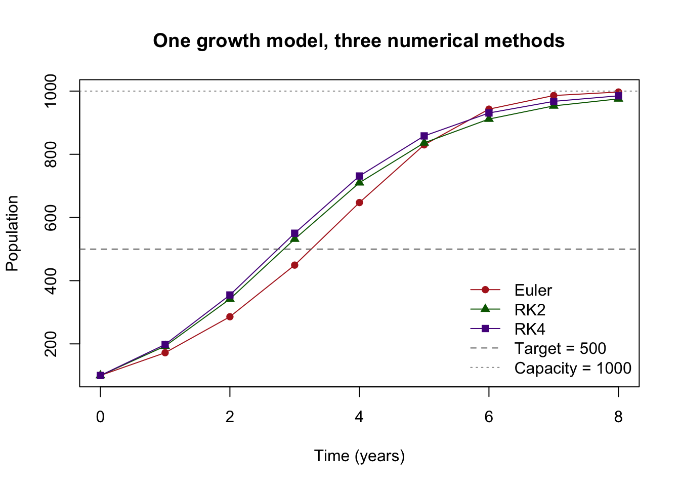
With one-year steps, Euler first records 500 or more at year 4, while RK2 and RK4 do so at year 3. This is a difference in the recorded threshold year; none of these values tells us the exact instant the population crosses 500 between observations. What would you tell someone who needs to plan for that milestone?

See the entire trajectory

plot(time, euler, type = "o", pch = 16, col = "firebrick",
     ylim = range(c(euler, rk2, rk4, capacity)),
     xlab = "Time (years)", ylab = "Population",
     main = "One growth model, three numerical methods")
lines(time, rk2, type = "o", pch = 17, col = "darkgreen")
lines(time, rk4, type = "o", pch = 15, col = "purple4")
abline(h = target, lty = 2, col = "gray40")
abline(h = capacity, lty = 3, col = "gray60")
legend("bottomright", c("Euler", "RK2", "RK4", "Target = 500", "Capacity = 1000"),
       col = c("firebrick", "darkgreen", "purple4", "gray40", "gray60"),
       lty = c(1, 1, 1, 2, 3), pch = c(16, 17, 15, NA, NA), bty = "n")

Do not just identify the smoothest line. Which method first reaches the target on our yearly grid? Do the methods move closer together later? What does the carrying-capacity line mean for the model?

Change the time step, not the model

Change only delta_t to 0.5 year, rerun the simulation and decision chunks, and record the three first times. Then try 2 years. Keep the same initial population, growth fraction, capacity, target, and eight-year endpoint.

\(\Delta t\) (years)	Euler first reaches 500	RK2 first reaches 500	RK4 first reaches 500
2	year 4	year 4	year 4
1	year 4	year 3	year 3
0.5	year 3.5	year 3	year 3

Why can the two-year grid make all three methods report year 4 even though their predicted populations differ? At \(\Delta t=2\), Euler even predicts a population above the carrying capacity by year 8. Is that a feature of the logistic model, or a warning about the numerical step?

Keep the two kinds of uncertainty separate

Smaller steps and a higher-order method can reduce numerical error for this equation. They cannot tell us whether \(r=0.8\), \(K=1000\), or even the logistic model is a good description of the real population. A precise solution to a poor model can still be a poor prediction.

If we have time: check against the exact model

For this particular logistic equation, the exact mathematical solution is

\[ P(t)=\frac{K}{1+(K/P_0-1)e^{-rt}}. \]

We do not need to derive it. Use it to check the methods at year 8, then say whether a tiny numerical error would change your confidence in the real-world forecast.

exact_at_8 <- capacity /
  (1 + (capacity / initial_population - 1) *
     exp(-growth_fraction * end_time))

data.frame(
  method = c("Euler", "RK2", "RK4"),
  estimate_at_year_8 = c(tail(euler, 1), tail(rk2, 1), tail(rk4, 1)),
  absolute_error = abs(c(tail(euler, 1), tail(rk2, 1),
                         tail(rk4, 1)) - exact_at_8)
)

  method estimate_at_year_8 absolute_error
1  Euler           997.0318      11.765518
2    RK2           975.4003       9.865975
3    RK4           985.0548       0.211517

If you changed the time step above, restore delta_t <- 1 and rerun the simulation to compare the original one-year results. At that step, the exact model predicts about 985.27 at year 8. Notice that RK4’s year-8 estimate is close to that value, but accuracy relative to the equation is not validation of the equation itself.