Runge-Kutta 4: Four Estimates of One Change

TipToday’s question

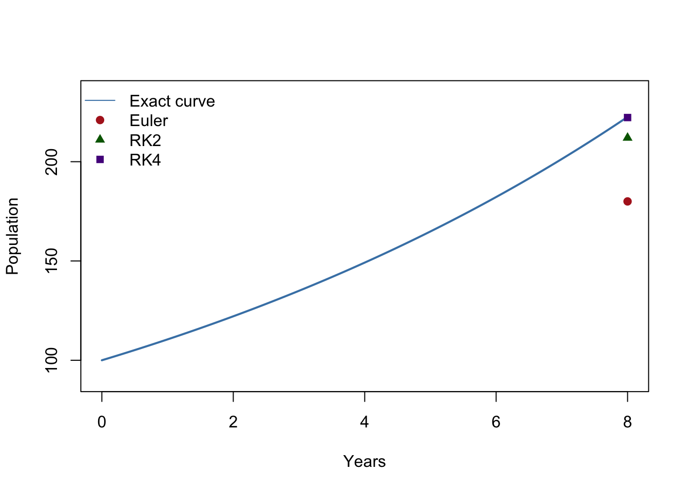
Euler samples the growth rate once per step. RK2 samples it twice. If we sample it four times—at the start, twice near the middle, and at the end—can we take a better step without changing our growth model?

NoteReading and code

Read Module 6.4, “Runge-Kutta 4 Method,” in Introduction to Computational Science. Download the complete R script after coding along. Project 3 still asks for Euler and RK2; RK4 is not required for that assignment.

Revisit the same eight-year step

Keep the model from Modules 6.2 and 6.3: \(P(0)=100\) and \(dP/dt=0.1P\) people per year. Let \(\Delta t=8\) years so we can see the difference among methods. We already found:

Method	Estimate at year 8
Euler	180
RK2	212
Exact solution, \(100e^{0.8}\)	about 222.55

Before we calculate: where do you expect RK4’s answer to land? Why? An answer closer to the exact model solution is not automatically a better prediction of a real population.

Four trial changes, all from the same starting value

The book calls these \(\partial_1,\partial_2,\partial_3,\partial_4\). Each is an estimate of the change over the full eight-year step, not a new population and not four successive steps. We will call them change_1 through change_4 in R.

First: use the starting rate

At \(P=100\), the rate is \(0.1(100)=10\) people/year. The first trial change is

\[ \partial_1=10(8)=80. \]

That is exactly Euler’s proposed change: \(100+80=180\).

Second: sample halfway along that trial

Half of the first change puts us at a trial population of \(100+80/2=140\) halfway through the interval. Its rate is \(0.1(140)=14\) people/year, giving a full-step trial change of

\[ \partial_2=14(8)=112. \]

Pause: why did we add only half of \(\partial_1\) to find the midpoint population, but multiply the midpoint rate by the full eight years to define \(\partial_2\)?

Third: try the midpoint again

Use half of the second change to find another trial midpoint: \(100+112/2=156\). Then

\[ \partial_3=0.1(156)(8)=124.8. \]

The third midpoint is different because its trial population came from \(\partial_2\), not \(\partial_1\).

Fourth: sample at a trial endpoint

Use the full third change to reach a trial endpoint population of \(100+124.8=224.8\). Then

\[ \partial_4=0.1(224.8)(8)=179.84. \]

ImportantThese are not four updates

We have not changed the stored population yet. All four rates are evaluated at trial values built from the same old population, 100. We update the stored population once, after combining the four changes.

Weight the trial changes

RK4 gives the two midpoint estimates twice as much weight as the endpoint estimates:

\[ \begin{aligned} \text{weighted change} &=\frac{\partial_1+2\partial_2+2\partial_3+\partial_4}{6}\\ &=\frac{80+2(112)+2(124.8)+179.84}{6}=122.24,\\ P_{\text{RK4}}(8)&=100+122.24=222.24. \end{aligned} \]

Compare 222.24 with Euler’s 180, RK2’s 212, and the exact model value of about 222.55. For this step, RK4 is closest. The weights are \(1,2,2,1\) divided by 6; we are not simply averaging four endpoint predictions.

old_population <- 100
growth_fraction <- 0.1       # per year
delta_t <- 8                 # years

change_1 <- growth_fraction * old_population * delta_t
change_2 <- growth_fraction * (old_population + change_1 / 2) * delta_t
change_3 <- growth_fraction * (old_population + change_2 / 2) * delta_t
change_4 <- growth_fraction * (old_population + change_3) * delta_t

data.frame(stage = c("start", "first midpoint", "second midpoint", "end"),
           trial_population = c(old_population,
                                old_population + change_1 / 2,
                                old_population + change_2 / 2,
                                old_population + change_3),
           full_step_change = c(change_1, change_2, change_3, change_4))

            stage trial_population full_step_change
1           start            100.0            80.00
2  first midpoint            140.0           112.00
3 second midpoint            156.0           124.80
4             end            224.8           179.84

weighted_change <- (change_1 + 2 * change_2 +
                    2 * change_3 + change_4) / 6
rk4_estimate <- old_population + weighted_change
rk4_estimate

[1] 222.24

Compare all four answers visually

smooth_time <- seq(0, 8, by = 0.1)
exact_curve <- 100 * exp(growth_fraction * smooth_time)

plot(smooth_time, exact_curve, type = "l", lwd = 2, col = "steelblue",
     xlab = "Years", ylab = "Population", ylim = c(90, 235))
points(c(8, 8, 8), c(180, 212, rk4_estimate),
       col = c("firebrick", "darkgreen", "purple4"), pch = c(19, 17, 15))
legend("topleft", c("Exact curve", "Euler", "RK2", "RK4"),
       col = c("steelblue", "firebrick", "darkgreen", "purple4"),
       lty = c(1, NA, NA, NA), pch = c(NA, 19, 17, 15), bty = "n")

General rule before we write the loop

If the rate is \(f(t,P)\), the four trial changes from an old point \((t,P)\) are:

\[ \begin{aligned} \partial_1 &= f(t,P)\Delta t,\\ \partial_2 &= f(t+\Delta t/2,\,P+\partial_1/2)\Delta t,\\ \partial_3 &= f(t+\Delta t/2,\,P+\partial_2/2)\Delta t,\\ \partial_4 &= f(t+\Delta t,\,P+\partial_3)\Delta t,\\ P_{\text{new}} &= P+(\partial_1+2\partial_2+2\partial_3+\partial_4)/6. \end{aligned} \]

Our growth rate \(0.1P\) does not depend explicitly on \(t\), so the R code only needs the trial populations. For a time-dependent rate, the second and third evaluations would use the midpoint time, and the fourth would use the endpoint time.

Repeat RK4 every two years

What should the first corrected value be with \(\Delta t=2\) years? Work through the four changes from \(P=100\) on paper or a whiteboard before running the loop. Then compare your result with the second row below.

initial_population <- 100
end_time <- 8
delta_t <- 2
time <- seq(0, end_time, by = delta_t)
population_rk4 <- numeric(length(time))
population_rk4[1] <- initial_population

for (i in 2:length(time)) {
  old_population <- population_rk4[i - 1]
  change_1 <- growth_fraction * old_population * delta_t
  change_2 <- growth_fraction * (old_population + change_1 / 2) * delta_t
  change_3 <- growth_fraction * (old_population + change_2 / 2) * delta_t
  change_4 <- growth_fraction * (old_population + change_3) * delta_t

  population_rk4[i] <- old_population +
    (change_1 + 2 * change_2 + 2 * change_3 + change_4) / 6
}

data.frame(time, population_rk4,
           exact = initial_population * exp(growth_fraction * time))

  time population_rk4    exact
1    0       100.0000 100.0000
2    2       122.1400 122.1403
3    4       149.1818 149.1825
4    6       182.2106 182.2119
5    8       222.5521 222.5541

The first two-year RK4 update is 122.14. At year 8, RK4 gives about 222.55208, while the exact solution is about 222.55409. Euler and RK2 with the same two-year step gave 207.36 and 221.5335, respectively.

exact_at_8 <- initial_population * exp(growth_fraction * end_time)
data.frame(method = c("Euler", "RK2", "RK4", "Exact"),
           estimate = c(207.36, 221.5335,
                        population_rk4[length(time)], exact_at_8),
           absolute_error = c(abs(207.36 - exact_at_8),
                              abs(221.5335 - exact_at_8),
                              abs(population_rk4[length(time)] - exact_at_8), 0))

  method estimate absolute_error
1  Euler 207.3600   15.194092849
2    RK2 221.5335    1.020592849
3    RK4 222.5521    0.002010271
4  Exact 222.5541    0.000000000

The first two estimates are results from our earlier modules; the RK4 estimate is calculated by the loop above. Why is it important to compare them at the same time step?

Accuracy has a cost—and a limit

Keep the model and end time fixed. Change only delta_t in the RK4 loop to 8, 1, and 0.5. Record the year-8 estimate and compare with the exact model solution:

\(\Delta t\) (years)	RK4 at year 8	Absolute error, approximately
8	222.240000	0.314093
2	222.552083	0.002010
1	222.553956	0.000137
0.5	222.554084	0.000009

For this smooth model, halving the step makes RK4’s error fall rapidly—roughly by a factor of 16 once the step is small enough. RK4 evaluates the rate four times per step, compared with two for RK2 and one for Euler. More numerical precision still cannot fix a poor growth-rate assumption or missing carrying capacity.

TipCheck your understanding

1. Why do change_2 and change_3 use different trial midpoint populations?
2. Why does change_4 use a full change_3, not half of it?
3. At what point in the loop is the stored population actually updated?
4. If measuring the real population has an uncertainty of about 10 people, what might be a reasonable stopping point for reducing numerical error?

If we have time: transfer the pattern

In Modules 6.2 and 6.3, we also used \(dP/dt=10+P/5\) with \(P(0)=500\) and \(\Delta t=0.1\). Without changing the four-stage structure, replace each growth_fraction * trial_population above with 10 + trial_population / 5. Which parts of the algorithm stay the same? This is optional practice, not a new requirement for Project 3.