Runge-Kutta 2: Predict, Then Correct

TipToday’s question

Euler uses the rate at the start of a step. What if the rate changes substantially before the step ends? We can predict an endpoint, estimate the rate there, and use the average of the two rates.

NoteReading and code

Read Module 6.3, “Runge-Kutta 2 Method,” in Introduction to Computational Science. This module calls the particular RK2 method here Euler’s predictor-corrector (EPC). Download the complete R script after coding along.

Start where Euler left off

We will reuse Module 6.2’s model: \(P(0)=100\) and \(dP/dt=0.1P\) people per year. Take one deliberately large, eight-year step so the difference between methods is easy to see.

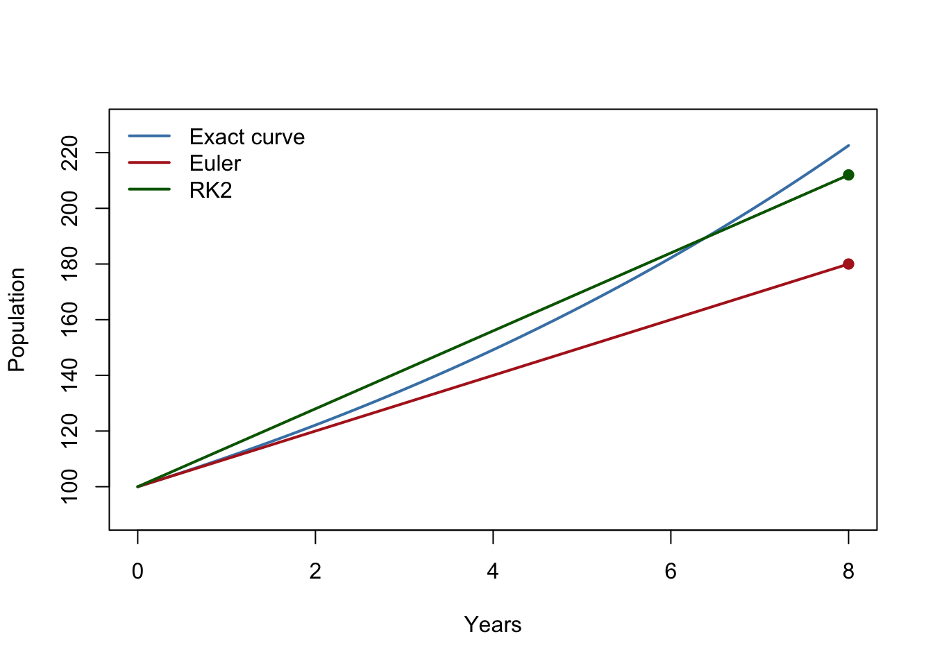
At the start, the rate is \(0.1(100)=10\) people/year. Euler predicts

\[ P_{\text{Euler}}(8)=100+10(8)=180. \]

This is a prediction, not yet our RK2 answer. The population is growing, so its rate at the end of the step is probably greater than 10. Before continuing, predict: should an improved estimate be above or below 180?

Correct the prediction

We do not know the actual population at year 8, so use Euler’s prediction of 180 to estimate the ending rate: \(0.1(180)=18\) people/year. Average the starting and predicted ending rates:

\[ \text{average rate}=\frac{10+18}{2}=14\text{ people/year}. \]

Now redo the step using that average:

\[ P_{\text{RK2}}(8)=100+14(8)=212. \]

The exact value for this particular model is \(100e^{0.8}\approx222.55\). For this large step, RK2 is closer than Euler, but it is not exact.

old_population <- 100
growth_fraction <- 0.1       # per year
delta_t <- 8                 # years

start_rate <- growth_fraction * old_population
euler_prediction <- old_population + start_rate * delta_t
predicted_end_rate <- growth_fraction * euler_prediction
average_rate <- (start_rate + predicted_end_rate) / 2
rk2_estimate <- old_population + average_rate * delta_t

exact_value <- old_population * exp(growth_fraction * delta_t)
data.frame(method = c("Euler", "RK2", "Exact"),
           year_8_population = c(euler_prediction, rk2_estimate, exact_value))

  method year_8_population
1  Euler          180.0000
2    RK2          212.0000
3  Exact          222.5541

ImportantKeep the two estimates separate

euler_prediction helps us find the second rate. We do not replace old_population with it. The corrected step still starts from the old population of 100.

See the difference

smooth_time <- seq(0, 8, by = 0.1)
exact_curve <- 100 * exp(growth_fraction * smooth_time)

plot(smooth_time, exact_curve, type = "l", lwd = 2, col = "steelblue",
     xlab = "Years", ylab = "Population", ylim = c(90, 230))
segments(0, 100, 8, euler_prediction, col = "firebrick", lwd = 2)
segments(0, 100, 8, rk2_estimate, col = "darkgreen", lwd = 2)
points(c(8, 8), c(euler_prediction, rk2_estimate),
       col = c("firebrick", "darkgreen"), pch = 19)
legend("topleft", c("Exact curve", "Euler", "RK2"),
       col = c("steelblue", "firebrick", "darkgreen"),
       lty = 1, lwd = 2, bty = "n")

The green segment uses an average rate, so it reaches a better endpoint here. It is still a straight-line approximation over the step; it is not the exact curved path.

Repeat the correction at every step

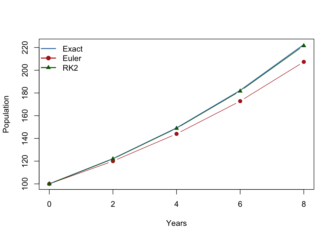
For several steps, each corrected value becomes the starting value of the next step. Use two-year steps from year 0 to year 8. First, calculate the next value by hand: what are the starting rate, Euler prediction, predicted ending rate, and corrected population after two years?

initial_population <- 100
end_time <- 8
delta_t <- 2
time <- seq(0, end_time, by = delta_t)
population_rk2 <- numeric(length(time))
population_rk2[1] <- initial_population

for (i in 2:length(time)) {
  old_population <- population_rk2[i - 1]
  start_rate <- growth_fraction * old_population
  euler_prediction <- old_population + start_rate * delta_t
  predicted_end_rate <- growth_fraction * euler_prediction
  average_rate <- (start_rate + predicted_end_rate) / 2
  population_rk2[i] <- old_population + average_rate * delta_t
}

data.frame(time, population_rk2)

  time population_rk2
1    0       100.0000
2    2       122.0000
3    4       148.8400
4    6       181.5848
5    8       221.5335

The first corrected value should be 122: start rate 10, predicted population 120, predicted end rate 12, average rate 11, and change \(11(2)=22\). Compare that hand calculation with the second row.

Compare with Euler at the same step size

population_euler <- numeric(length(time))
population_euler[1] <- initial_population

for (i in 2:length(time)) {
  old_population <- population_euler[i - 1]
  rate_now <- growth_fraction * old_population
  population_euler[i] <- old_population + rate_now * delta_t
}

plot(time, initial_population * exp(growth_fraction * time),
     type = "l", lwd = 2, col = "steelblue",
     xlab = "Years", ylab = "Population")
lines(time, population_euler, type = "b", col = "firebrick", pch = 19)
lines(time, population_rk2, type = "b", col = "darkgreen", pch = 17)
legend("topleft", c("Exact", "Euler", "RK2"),
       col = c("steelblue", "firebrick", "darkgreen"),
       lty = 1, pch = c(NA, 19, 17), lwd = 2, bty = "n")

data.frame(method = c("Euler", "RK2", "Exact"),
           year_8_population = c(population_euler[length(time)],
                                 population_rk2[length(time)],
                                 initial_population * exp(growth_fraction * end_time)))

  method year_8_population
1  Euler          207.3600
2    RK2          221.5335
3  Exact          222.5541

With two-year steps, Euler estimates 207.36 and RK2 estimates about 221.53 at year 8; the exact value is about 222.55.

Does the time step still matter?

Predict what will happen to both methods if we shorten the step. Then change delta_t above to 8, 1, and 0.5 and rerun the two loops, keeping the model and end time fixed.

Step, years	Euler at year 8	RK2 at year 8	Exact at year 8
8	180.00	212.00	222.55
2	207.36	221.53	222.55
1	214.36	222.28	222.55
0.5	218.29	222.48	222.55

For this smooth model and these step sizes, RK2 has less numerical error than Euler at the same step size. It uses two rate evaluations per step instead of one. A better numerical answer does not prove that \(0.1P\) accurately describes a real population.

TipCheck your understanding

1. In the loop, which value is the predictor, and which is the corrected population?
2. Why must predicted_end_rate use euler_prediction, not old_population?
3. If the rate also depended explicitly on time, at which time would you evaluate the second rate?
4. Could a smaller Euler step outperform a much larger RK2 step? What comparison would you run?

Try a different rate from the book

Module 6.3’s Quick Review Question 1 returns to \(dP/dt=10+P/5\), starting at \(P=500\), with a step of \(0.1\). Predict the corrected value before running this code. The Euler prediction is 511; what ending rate does that predict?

old_population <- 500
delta_t <- 0.1

start_rate <- 10 + old_population / 5
euler_prediction <- old_population + start_rate * delta_t
predicted_end_rate <- 10 + euler_prediction / 5
corrected_population <- old_population +
  (start_rate + predicted_end_rate) / 2 * delta_t

data.frame(start_rate, euler_prediction,
           predicted_end_rate, corrected_population)

  start_rate euler_prediction predicted_end_rate corrected_population
1        110              511              112.2               511.11

The corrected result is 511.11. The sequence is the same for any rate formula: start rate → Euler prediction → predicted end rate → average rate → corrected update. This particular predictor-corrector scheme is one version of RK2, not the only possible RK2 formula.