We have used old amount + rate × time step in every simulation so far. Why does that update make sense, and how much can the answer change when we choose a different time step?
NoteReading and code
Read Module 6.2, “Euler’s Method,” in Introduction to Computational Science. Download the complete R script after coding along.
The update we already know
Suppose a population \(P\) grows at an instantaneous rate of \(0.1P\) individuals per year. At the moment when \(P=100\), its rate is 10 individuals per year. Euler’s method assumes that current rate stays constant for one short time step:
\[
P_{\text{new}}=P_{\text{old}}+\underbrace{(0.1P_{\text{old}})}_{\text{rate at the old value}}\Delta t.
\]
The rate is the slope of the population curve at the starting point. Euler follows a straight tangent line for one step, then finds a new slope and repeats. It does not know the future slope in advance.
Predict one very large step
Start at \(P(0)=100\) and jump all the way to year 8 in one step. What would Euler predict? The starting slope is \(0.1(100)=10\) individuals/year, so
\[
P_{\text{Euler}}(8)=100+10(8)=180.
\]
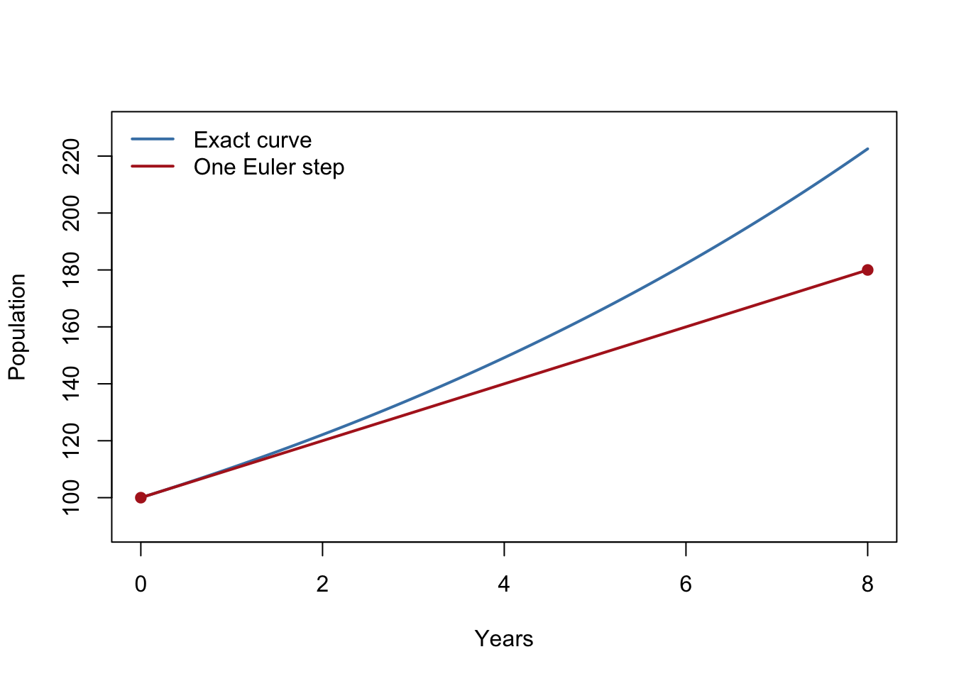
For this particular model, we also know the exact solution \(P(t)=100e^{0.1t}\). It gives about 222.55 at year 8. The large Euler step falls short because the true curve bends upward while Euler keeps the starting slope of 10 for all eight years.
initial_population <-100growth_fraction <-0.1# per yearend_time <-8# yearsdelta_t <-8# one very large stepold_population <- initial_populationgrowth_rate <- growth_fraction * old_populationeuler_estimate <- old_population + growth_rate * delta_texact_value <- initial_population *exp(growth_fraction * end_time)euler_estimate
[1] 180
exact_value
[1] 222.5541
abs(euler_estimate - exact_value)
[1] 42.55409
See the tangent-line estimate
The blue curve is the exact solution. The red segment shows the one-step Euler estimate. Where do the two paths begin to separate?
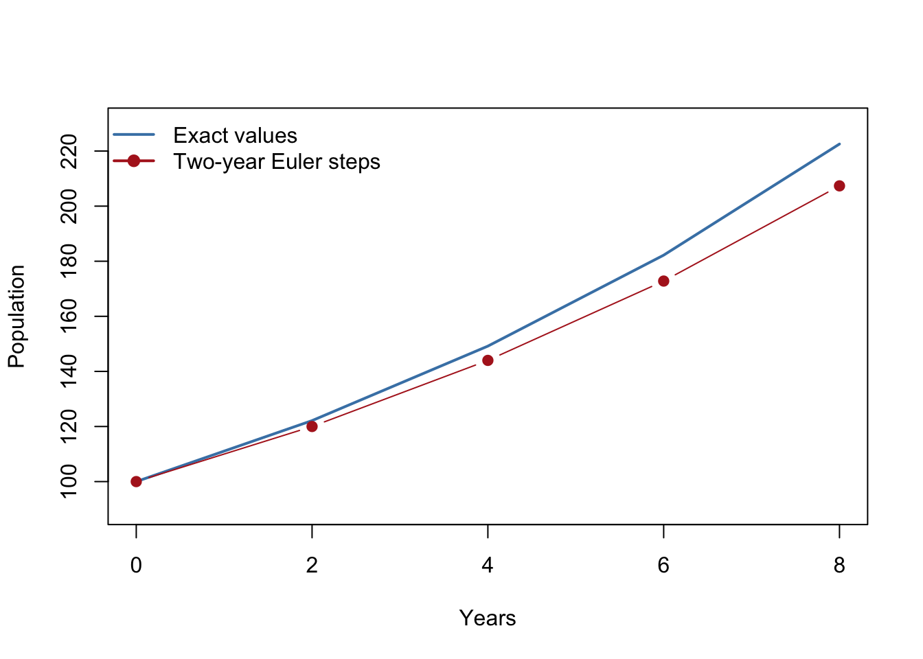
Now use four steps of two years each. Before running the loop, predict the first two estimates. The first is \(100+0.1(100)(2)=120\). For the second, use the new starting value of 120 to find a new slope: \(120+0.1(120)(2)=144\).
Inside the loop, the rate must be computed from population[i - 1], the population at the start of that step. Updating the population and then using the new value to compute the same step’s rate would be a different method.
How small should a step be?
Change only delta_t in the loop above to 8, 1, and 0.5. Keep the same initial population, rate, and final time. Record the final estimate and its absolute error against the exact value. The book’s Module 6.2 asks us to compare solutions this way.
\(\Delta t\) (years)
Steps to year 8
Euler estimate at year 8
Absolute error, approximately
8
1
180.000
42.554
2
4
207.360
15.194
1
8
214.359
8.195
0.5
16
218.287
4.267
Smaller steps improve this particular approximation, but require more calculations. Halving the step from 1 to 0.5 roughly halves the error here—an example of Euler’s first-order behavior. That pattern is not a promise for every model or every step size. It also says nothing by itself about whether \(0.1P\) is a good model of a real population.
TipCheck your interpretation
Which error can we reduce by shrinking \(\Delta t\): an incorrect growth-rate estimate, a missing carrying capacity, or the finite-step approximation?
If the model is wrong, could a more accurate numerical method still produce the wrong real-world prediction?
How many times does the loop update the population when \(\Delta t=0.5\) over eight years?
Transfer the method to a different rate
Euler’s update is not limited to proportional growth. In the book’s Quick Review Question 1, the rate is \(10+P/5\), the initial population is 500, and \(\Delta t=0.1\). Find the rate at the old value, multiply by the step, and add it. Predict the first estimate before running R.
  time population
1  0.0     500.00
2  0.1     511.00
3  0.2     522.22
The first estimate is 511; the second is 522.22. The only part of the loop that changed was the formula for the rate. That is the core of Euler’s method: start with the current value, estimate a change using the current slope, then step forward.