flowchart LR
  S[Susceptible S] -->|infection flow: beta S I| I[Infectious I]
  I -->|recovery flow: gamma I| R[Recovered R]
flowchart LR S[Susceptible S] -->|infection flow: beta S I| I[Infectious I] I -->|recovery flow: gamma I| R[Recovered R]
After this module, you should be able to:
A closed population contains 762 susceptible people and one infectious person. Initially, no one has recovered.
The population is divided into three stocks:
| Stock | Meaning |
|---|---|
| \(S\) | susceptible: can become infected |
| \(I\) | infectious: currently able to transmit infection |
| \(R\) | recovered/removed: no longer infectious and cannot be infected again in this model |
For our simulation, removal means recovery with lasting immunity. Births, deaths, and migration are omitted, so the total population \(N=S+I+R\) stays constant.
flowchart LR
  S[Susceptible S] -->|infection flow: beta S I| I[Infectious I]
I -->|recovery flow: gamma I| R[Recovered R]flowchart LR S[Susceptible S] -->|infection flow: beta S I| I[Infectious I] I -->|recovery flow: gamma I| R[Recovered R]
Unlike predator–prey, an infection does not create another person. It transfers someone from \(S\) to \(I\). Recovery transfers someone from \(I\) to \(R\).
Write the infection flow as \(\beta SI\) and the recovery flow as \(\gamma I\):
\[ \frac{dS}{dt}=-\beta SI, \qquad \frac{dI}{dt}=\beta SI-\gamma I, \qquad \frac{dR}{dt}=\gamma I. \]
| Parameter | Meaning | Units in this formulation |
|---|---|---|
| \(\beta\) | transmission coefficient: converts susceptible–infectious encounters into new infections | per person per day |
| \(\gamma\) | recovery rate per infectious person | per day |
| \(\Delta t\) | time step | days |
The product \(SI\) represents potential encounters under a well-mixed population assumption. The transmission coefficient summarizes contact and transmission effects; it is not by itself a probability.
With \(\gamma=0.5\) per day, the average infectious duration in this model is \(1/\gamma=2\) days. Recovery happens continuously at rate \(\gamma I\); the model does not say every person recovers exactly two days after infection.
Use \(S=762\), \(I=1\), \(R=0\), \(\beta=0.00218\), \(\gamma=0.5\), and \(\Delta t=0.01\) day.
\[ \text{infection flow}=0.00218(762)(1)=1.66116 \]
\[ \text{recovery flow}=0.5(1)=0.5 \]
Both flows have units of people per day. Over the first time step,
\[ S_{new}=762-1.66116(0.01)=761.9833884, \]
\[ I_{new}=1+(1.66116-0.5)(0.01)=1.0116116, \]
\[ R_{new}=0+0.5(0.01)=0.005. \]
Their sum is still 763. Fractional people are expected in this continuous model.
These are the parameters from our earlier SIR example. We extend the simulation to 28 days to see more of the outbreak’s decline.
delta_t <- 0.01                  # days per step
end_time <- 28                   # days
time <- seq(0, end_time, by = delta_t)

transmission_coefficient <- 0.00218  # per person per day
recovery_rate <- 0.5                # per day

initial_susceptible <- 762
initial_infectious <- 1
initial_recovered <- 0
total_population <- initial_susceptible +
initial_infectious + initial_recoveredsusceptible <- numeric(length(time))
infectious <- numeric(length(time))
recovered <- numeric(length(time))
susceptible[1] <- initial_susceptible
infectious[1] <- initial_infectious
recovered[1] <- initial_recoveredfor (i in 2:length(time)) {
susceptible_old <- susceptible[i - 1]
infectious_old <- infectious[i - 1]
recovered_old <- recovered[i - 1]
infection_flow <- transmission_coefficient *
susceptible_old * infectious_old
recovery_flow <- recovery_rate * infectious_old
susceptible[i] <- susceptible_old - infection_flow * delta_t
infectious[i] <- infectious_old +
(infection_flow - recovery_flow) * delta_t
recovered[i] <- recovered_old + recovery_flow * delta_t
}Calculate both flows from the old values, then apply exactly the same transfer to the group that loses people and the group that gains them.
results <- data.frame(time, susceptible, infectious, recovered)
results$total <- results$susceptible +
  results$infectious + results$recovered

head(results)
time susceptible infectious recovered total
1 0.00 762.0000 1.000000 0.00000000 763
2 0.01 761.9834 1.011612 0.00500000 763
3 0.02 761.9666 1.023358 0.01005806 763
4 0.03 761.9496 1.035240 0.01517485 763
5 0.04 761.9324 1.047259 0.02035105 763
6 0.05 761.9150 1.059418 0.02558734 763range(results$total)[1] 763 763max(abs(results$total - total_population))[1] 2.16005e-12Check the first updated row against the hand calculation. The total should stay at 763 apart from tiny floating-point rounding differences. Population conservation is a useful check on the code, although it does not establish that the assumptions describe a real outbreak.
plot(
  time,
  susceptible,
  type = "l",
  lwd = 3,
  col = "#214f73",
  ylim = c(0, total_population),
  xlab = "Time (days)",
  ylab = "People",
  main = "A simulated SIR outbreak"
)
lines(time, infectious, lwd = 3, col = "#b65335")
lines(time, recovered, lwd = 3, lty = 2, col = "#276b55")
legend(
  "right",
  legend = c("Susceptible", "Infectious", "Recovered"),
  col = c("#214f73", "#b65335", "#276b55"),
  lty = c(1, 1, 2),
  lwd = c(3, 3, 3),
  bty = "n"
)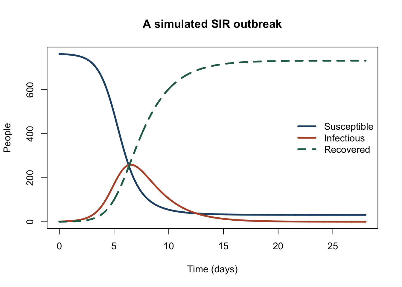
Susceptible people can only leave their group, recovered people can only enter theirs, and the infectious population has both an inflow and an outflow. That is why \(I\) can rise and then fall.
peak_position <- which.max(results$infectious)
results[peak_position, ]
time susceptible infectious recovered total
655 6.54 228.8186 258.8071 275.3743 763This reports the largest infectious population in the simulated interval, together with its time and the other groups at that moment.
The people who have ever been infected include both those still infectious and those now recovered:
last_position <- length(time)
ever_infected <- infectious[last_position] + recovered[last_position]
fraction_infected <- ever_infected / total_population

tail(results, 1)
time susceptible infectious recovered total
2801 28 31.17163 0.04816407 731.7802 763ever_infected[1] 731.8284fraction_infected[1] 0.959146This calculation works here because no one starts in the recovered group and there are no repeat infections. It is a cumulative count by day 28, rather than a claim that the outbreak has ended exactly at that time.
Factor the infectious equation:
\[ \frac{dI}{dt}=I(\beta S-\gamma). \]
For \(I>0\), infections increase when \(\beta S>\gamma\) and decrease when \(\beta S<\gamma\). The turning point is near
\[ S^*=\frac{\gamma}{\beta}. \]
susceptible_threshold <- recovery_rate / transmission_coefficient
susceptible_threshold
[1] 229.3578results[peak_position, ] time susceptible infectious recovered total
655 6.54 228.8186 258.8071 275.3743 763Infections can decline while susceptible people remain: the infection flow has become smaller than the recovery flow.
For a fully susceptible population of size \(N\), this model’s basic reproduction number is
\[ \mathcal{R}_0=\frac{\beta N}{\gamma}. \]
At a particular time, the effective reproduction number is
\[ \mathcal{R}_{eff}(t)=\frac{\beta S(t)}{\gamma}. \]
basic_reproduction_number <- transmission_coefficient *
  total_population / recovery_rate
results$effective_reproduction_number <- transmission_coefficient *
  results$susceptible / recovery_rate

basic_reproduction_number
[1] 3.32668results[c(1, peak_position, last_position), ] time susceptible infectious recovered total
1 0.00 762.00000 1.00000000 0.0000 763
655 6.54 228.81862 258.80709371 275.3743 763
2801 28.00 31.17163 0.04816407 731.7802 763
effective_reproduction_number
1 3.3223200
655 0.9976492
2801 0.1359083A value greater than 1 supports increasing infections; a value less than 1 supports decreasing infections in this model. The basic reproduction number assumes everyone is susceptible, while the effective number changes as the susceptible pool shrinks. Neither is a permanent property of a disease independent of population and contact assumptions.
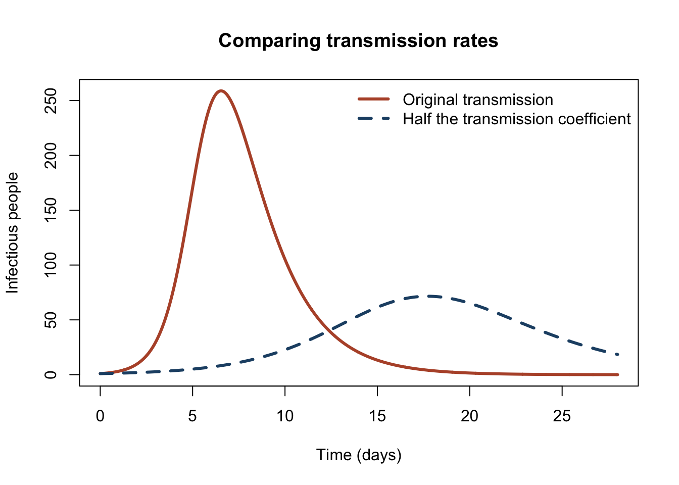
Suppose the transmission coefficient is half as large from the beginning. Predict whether this will prevent growth completely or produce a smaller outbreak. Check the initial effective reproduction number before running the experiment.
reduced_transmission <- transmission_coefficient / 2
reduced_transmission * initial_susceptible / recovery_rate
[1] 1.66116reduced_susceptible <- numeric(length(time))
reduced_infectious <- numeric(length(time))
reduced_recovered <- numeric(length(time))
reduced_susceptible[1] <- initial_susceptible
reduced_infectious[1] <- initial_infectious
reduced_recovered[1] <- initial_recovered
for (i in 2:length(time)) {
susceptible_old <- reduced_susceptible[i - 1]
infectious_old <- reduced_infectious[i - 1]
recovered_old <- reduced_recovered[i - 1]
infection_flow <- reduced_transmission *
susceptible_old * infectious_old
recovery_flow <- recovery_rate * infectious_old
reduced_susceptible[i] <- susceptible_old - infection_flow * delta_t
reduced_infectious[i] <- infectious_old +
(infection_flow - recovery_flow) * delta_t
reduced_recovered[i] <- recovered_old + recovery_flow * delta_t
}plot(
time,
infectious,
type = "l",
lwd = 3,
col = "#b65335",
ylim = c(0, max(infectious, reduced_infectious)),
xlab = "Time (days)",
ylab = "Infectious people",
main = "Comparing transmission rates"
)
lines(time, reduced_infectious, lwd = 3, lty = 2, col = "#214f73")
legend(
"topright",
legend = c("Original transmission", "Half the transmission coefficient"),
col = c("#b65335", "#214f73"),
lty = c(1, 2),
lwd = c(3, 3),
bty = "n"
)
reduced_peak_position <- which.max(reduced_infectious)
data.frame(
  scenario = c("Original", "Reduced transmission"),
  peak_infectious = c(infectious[peak_position],
    reduced_infectious[reduced_peak_position]),
  peak_day = c(time[peak_position], time[reduced_peak_position]),
  infected_by_day_28 = c(ever_infected,
    reduced_infectious[last_position] + reduced_recovered[last_position])
)
scenario peak_infectious peak_day infected_by_day_28
1 Original 258.80709 6.54 731.8284
2 Reduced transmission 71.54104 17.72 491.1648The same 28-day window makes the comparison consistent, but an outbreak with slower transmission may still be active at the end. Extend the time horizon before comparing eventual outbreak sizes.
The textbook’s SARS model adds detail to address processes that SIR combines or omits:
Each addition introduces a stock, a transfer, or a changed contact rate. The coding principle stays the same: calculate flows from the old state, then apply them consistently to every affected stock. Begin by drawing the transfers before attempting a larger model.
The SIR simulation here is a simplified teaching example, not a fitted SARS model. Its parameters come from the earlier course’s SIR example; the SARS extension has different assumptions and parameters.
The basic SIR model assumes a closed, well-mixed population; constant transmission and recovery rates; immediate infectiousness after infection; lasting immunity; and continuous deterministic flows.
Predict, then test:
if statement inside the loop.