delta_t <- 0.01                # months per step
end_time <- 12                 # months
time <- seq(0, end_time, by = delta_t)

squirrel_birth_rate <- 2       # per month
predation_effect <- 0.02       # effect of each hawk on squirrels
hawk_growth_effect <- 0.01     # effect of each squirrel on hawks
hawk_death_rate <- 1.06        # per month

squirrels <- numeric(length(time))
hawks <- numeric(length(time))
squirrels[1] <- 100
hawks[1] <- 15Learning goals
After this module, you should be able to:
- explain how predator–prey interaction differs from competition;
- identify the signs and units of four model flows;
- calculate one Euler step by hand;
- update both populations from their values at the same time;
- interpret population graphs and a predator-versus-prey graph; and
- describe what the model leaves out.
Predict before coding
Imagine 100 squirrels and 15 hawks in an isolated habitat.
- What happens to hawks if squirrels become scarce?
- If squirrels increase first, will hawks increase immediately or later?
- Could both populations rise and fall repeatedly?
Sketch two possible population graphs. We will compare them with a simulation.
One interaction, opposite effects
In Module 4.1, an encounter between species reduced both populations’ growth. Here an encounter harms the prey and benefits the predator.
Let \(S\) be the number of squirrels and \(H\) the number of hawks. The model is
\[ \frac{dS}{dt}=aS-bSH \]
and
\[ \frac{dH}{dt}=cSH-dH. \]
| Flow | Formula | Effect |
|---|---|---|
| squirrel births | \(aS\) | squirrels increase |
| squirrels lost to predation | \(bSH\) | squirrels decrease |
| hawk growth supported by prey | \(cSH\) | hawks increase |
| hawk deaths | \(dH\) | hawks decrease |
The interaction term \(SH\) is zero if either species is absent. It represents potential encounters under a well-mixed population assumption. The constants \(b\) and \(c\) translate those encounters into effects on the two populations; they are not probabilities of one particular squirrel being eaten or one hawk being born.
The terms \(a\) and \(d\) have units per month. The interaction constants \(b\) and \(c\) have units that make \(bSH\) and \(cSH\) rates in animals per month; informally, they are per animal per month. Model populations are continuous quantities, even though real animals come in whole numbers.
Check one step by hand
Use the values from our older squirrel–hawk example:
| Quantity | Value |
|---|---|
| initial squirrels \(S_0\) | 100 |
| initial hawks \(H_0\) | 15 |
| squirrel birth rate \(a\) | 2 per month |
| predation effect on squirrels \(b\) | 0.02 per hawk per month |
| prey effect on hawks \(c\) | 0.01 per squirrel per month |
| hawk death rate \(d\) | 1.06 per month |
| time step \(\Delta t\) | 0.01 month |
At the beginning, the squirrel change rate is
\[ 2(100)-0.02(100)(15)=200-30=170 \]
squirrels per month. The hawk change rate is
\[ 0.01(100)(15)-1.06(15)=15-15.9=-0.9 \]
hawks per month. During the first step,
\[ S_{new}=100+170(0.01)=101.7, \qquad H_{new}=15-0.9(0.01)=14.991. \]
An initially decreasing hawk population can increase later if squirrels become abundant.
Build the simulation in R
1. Time, parameters, and initial conditions
2. Advance both populations together
for (i in 2:length(time)) {
  squirrels_old <- squirrels[i - 1]
  hawks_old <- hawks[i - 1]

  squirrel_births <- squirrel_birth_rate * squirrels_old
  squirrels_eaten <- predation_effect * squirrels_old * hawks_old
  hawk_growth <- hawk_growth_effect * squirrels_old * hawks_old
  hawk_deaths <- hawk_death_rate * hawks_old

  squirrels[i] <- squirrels_old +
    (squirrel_births - squirrels_eaten) * delta_t
  hawks[i] <- hawks_old +
    (hawk_growth - hawk_deaths) * delta_t
}
Both updates use squirrels_old and hawks_old. A new value from this step must not be fed into the other species’ update for the same step.
3. Verify before interpreting
results <- data.frame(time, squirrels, hawks)
head(results)
time squirrels hawks
1 0.00 100.0000 15.00000
2 0.01 101.7000 14.99100
3 0.02 103.4291 14.98455
4 0.03 105.1877 14.98070
5 0.04 106.9763 14.97948
6 0.05 108.7953 14.98095Check the second row against 101.7 squirrels and 14.991 hawks. Then look at the last few rows and the population ranges:
tail(results) time squirrels hawks
1196 11.95 313.9781 19.34450
1197 11.96 319.0429 19.74683
1198 11.97 324.1637 20.16752
1199 11.98 329.3395 20.60750
1200 11.99 334.5689 21.06775
1201 12.00 339.8505 21.54929range(results$squirrels)[1] 3.681251 512.569409range(results$hawks)[1] 11.31443 348.00830Graph the populations over time
plot(
  time,
  squirrels,
  type = "l",
  lwd = 3,
  col = "#276b55",
  ylim = c(0, max(squirrels, hawks)),
  xlab = "Time (months)",
  ylab = "Population",
  main = "Squirrels and hawks over time"
)
lines(time, hawks, lwd = 3, lty = 2, col = "#b65335")
legend(
  "topright",
  legend = c("Squirrels", "Hawks"),
  col = c("#276b55", "#b65335"),
  lty = c(1, 2),
  lwd = c(3, 3),
  bty = "n"
)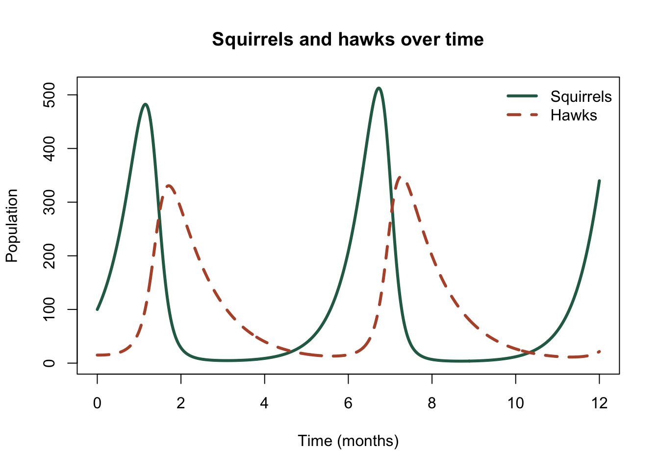
Where do the squirrel and hawk populations turn around? Does the predator response appear to lag behind the prey response? A plot suggests an answer; the numerical output lets us check it.
squirrel_peak_position <- which.max(squirrels)
hawk_peak_position <- which.max(hawks)

results[squirrel_peak_position, ]
time squirrels hawks
674 6.73 512.5694 102.8439results[hawk_peak_position, ] time squirrels hawks
728 7.27 102.8613 348.0083These are the largest peaks in the chosen 12-month window. Change the window and the reported peaks may change.
Graph predators against prey
Instead of placing time on the horizontal axis, plot one population against the other:
plot(
  squirrels,
  hawks,
  type = "l",
  lwd = 2,
  col = "#6b4c8a",
  xlab = "Squirrels",
  ylab = "Hawks",
  main = "A predator-prey trajectory"
)
points(squirrels[1], hawks[1], pch = 19, col = "#b65335")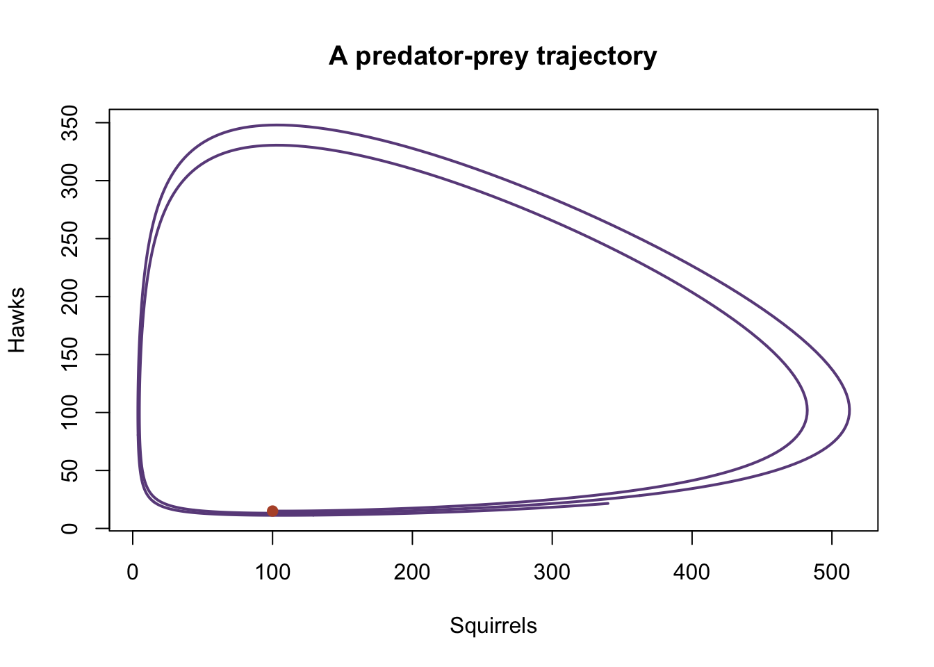
The point marks the initial state. A looping path means the two populations pass through different combinations as they rise and fall. The graph does not itself tell us how much time passes between points; keep the time-series graph alongside it.
Equilibrium and model limits
A coexistence equilibrium requires both rates of change to be zero. For positive populations,
\[ H^*=\frac{a}{b}=\frac{2}{0.02}=100, \qquad S^*=\frac{d}{c}=\frac{1.06}{0.01}=106. \]
equilibrium_squirrels <- hawk_death_rate / hawk_growth_effect
equilibrium_hawks <- squirrel_birth_rate / predation_effect

equilibrium_squirrels
[1] 106equilibrium_hawks[1] 100Our initial state is different, so the populations move. The classic model also assumes unlimited prey growth when hawks are absent, constant rates, no migration, and immediate effects of encounters. Its oscillations are a useful hypothesis about interaction, not a forecast for a real habitat. Euler’s method adds numerical error; try a smaller delta_t if the trajectory looks sensitive to the step size.
Further experiments
Predict before changing the code.
- Start with 25 hawks. Which population changes direction first?
- Increase
hawk_death_rate. How do the population peaks shift? - Set
hawks[1] <- 0. What happens to each population, and which assumption becomes most questionable? - Double
delta_tand compare results at the same times.
What to remember
- Predator–prey models use two coupled stocks and four flows.
- Encounters reduce prey and support predator growth.
- Use both old population values when calculating each new step.
- Population peaks can occur at different times.
- A plausible curve does not by itself validate the ecological assumptions.