delta_t <- 0.01
end_time <- 5
time <- seq(0, end_time, by = delta_t)

whitetip_birth_fraction <- 1
blacktip_birth_fraction <- 1
whitetip_competition_constant <- 0.27
blacktip_competition_constant <- 0.20Learning goals
After working through this module, you should be able to:
- distinguish competition from other ecological interactions;
- explain why an interaction term contains both populations;
- translate two coupled differential equations into Euler updates;
- simulate and graph two stocks in R;
- use results to determine which species persists; and
- identify important limitations of a simple competition model.
From one stock to two
In Modules 2.2 and 2.3, one population changed over time. Competition requires two stock variables because each population affects the other.
| Interaction | Effect on species 1 | Effect on species 2 |
|---|---|---|
| mutualism | + | + |
| predator-prey | + | - |
| competition | - | - |
The minus signs do not mean that both populations must decrease at every moment. Each species may still reproduce. Competition adds a negative flow to each population.
The shark scenario
Whitetip sharks and blacktip sharks compete for limited resources. Let
- \(W\) be the whitetip shark population;
- \(B\) be the blacktip shark population;
- \(a\) and \(b\) be their proportional birth rates; and
- \(c\) and \(d\) measure the effects of interspecies competition.
The model is
\[ \frac{dW}{dt}=aW-cWB \]
and
\[ \frac{dB}{dt}=bB-dBW. \]
The parameters from the earlier shark example are:
| Parameter | Value | Meaning |
|---|---|---|
| \(a\) | 1 per month | whitetip births per whitetip |
| \(b\) | 1 per month | blacktip births per blacktip |
| \(c\) | 0.27 per blacktip per month | effect of blacktips on each whitetip |
| \(d\) | 0.20 per whitetip per month | effect of whitetips on each blacktip |
| \(W_0\) | 20 sharks | initial whitetip population |
| \(B_0\) | 15 sharks | initial blacktip population |
Why multiply the populations?
The interaction terms are proportional to \(WB\).
- If either species is absent, \(WB=0\), so interspecies competition disappears.
- Doubling one population doubles the number of potential interactions.
- Doubling both populations multiplies potential interactions by four.
This is a mass-action assumption: the populations are well mixed, and encounters are proportional to the product of their sizes.
Check one step by hand
Use \(W=20\), \(B=15\), and \(\Delta t=0.01\) month.
For whitetips:
\[ \text{births}=1(20)=20 \]
\[ \text{competition deaths}=0.27(20)(15)=81 \]
\[ W_{new}=20+(20-81)(0.01)=19.39. \]
For blacktips:
\[ \text{births}=1(15)=15 \]
\[ \text{competition deaths}=0.20(15)(20)=60 \]
\[ B_{new}=15+(15-60)(0.01)=14.55. \]
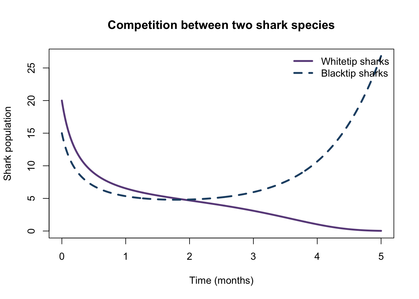
Both populations initially decrease, but that does not tell us what will happen later. As one population changes, it changes the competitive pressure on the other.
Build the simulation in R
1. Set up time and parameters
2. Create and initialize both stocks
whitetips <- numeric(length(time))
blacktips <- numeric(length(time))

whitetips[1] <- 20
blacktips[1] <- 15
3. Update both populations from the old values
for (i in 2:length(time)) {
  whitetips_old <- whitetips[i - 1]
  blacktips_old <- blacktips[i - 1]

  whitetip_births <- whitetip_birth_fraction * whitetips_old
  blacktip_births <- blacktip_birth_fraction * blacktips_old

  whitetip_competition_deaths <- whitetip_competition_constant *
    whitetips_old * blacktips_old
  blacktip_competition_deaths <- blacktip_competition_constant *
    blacktips_old * whitetips_old

  whitetips[i] <- whitetips_old +
    (whitetip_births - whitetip_competition_deaths) * delta_t
  blacktips[i] <- blacktips_old +
    (blacktip_births - blacktip_competition_deaths) * delta_t
}4. Organize and verify the results
shark_results <- data.frame(
  time,
  whitetips,
  blacktips
)

head(shark_results)
time whitetips blacktips
1 0.00 20.00000 15.00000
2 0.01 19.39000 14.55000
3 0.02 18.82216 14.13125
4 0.03 18.29224 13.74060
5 0.04 17.79652 13.37532
6 0.05 17.33180 13.03300The second row should agree with our hand calculation: about 19.39 whitetips and 14.55 blacktips.
5. Graph both populations
plot(
  time,
  whitetips,
  type = "l",
  lwd = 3,
  col = "#6b4c8a",
  ylim = c(0, max(whitetips, blacktips)),
  xlab = "Time (months)",
  ylab = "Shark population",
  main = "Competition between two shark species"
)
lines(time, blacktips, lwd = 3, lty = 2, col = "#214f73")
legend(
  "topright",
  legend = c("Whitetip sharks", "Blacktip sharks"),
  col = c("#6b4c8a", "#214f73"),
  lty = c(1, 2),
  lwd = c(3, 3),
  bty = "n"
)
Use the model to answer questions
When do whitetips fall below one shark?
below_one <- which(shark_results$whitetips < 1)[1]
shark_results[c(below_one - 1, below_one), ]
time whitetips blacktips
402 4.01 1.002961 10.75393
403 4.02 0.983869 10.83989The model uses continuous quantities, so “less than one shark” is a useful extinction threshold rather than a literal fractional animal.
Which species persists over this five-month run?
tail(shark_results) time whitetips blacktips
496 4.95 0.03407758 25.53382
497 4.96 0.03206901 25.78742
498 4.97 0.03015686 26.04364
499 4.98 0.02833786 26.30251
500 4.99 0.02660878 26.56404
501 5.00 0.02496641 26.82827Blacktips persist while whitetips approach zero. Notice that the blacktip population begins growing rapidly once competition from whitetips becomes weak.
Equilibria
A nonzero equilibrium requires both rates of change to equal zero:
\[ a-cB=0 \qquad\text{and}\qquad b-dW=0. \]
Therefore,
\[ B^*=\frac{a}{c}=\frac{1}{0.27}\approx3.70 \]
and
\[ W^*=\frac{b}{d}=\frac{1}{0.20}=5. \]
equilibrium_blacktips <- whitetip_birth_fraction /
  whitetip_competition_constant
equilibrium_whitetips <- blacktip_birth_fraction /
  blacktip_competition_constant

equilibrium_whitetips
[1] 5equilibrium_blacktips[1] 3.703704Starting exactly at this pair keeps the populations constant in the model. Small changes can push the system toward a different outcome, so this coexistence equilibrium is not necessarily stable.
Assumptions and limitations
This model assumes:
- each species would grow exponentially without the competitor;
- competition depends only on encounters between the two species;
- the environment is well mixed;
- all sharks of a species are interchangeable;
- parameters remain constant; and
- migration, age structure, randomness, and delays are negligible.
The winning population can eventually grow without bound because the model includes no within-species carrying capacity. That is a warning about long-term use, not a coding error. A richer model could constrain each species as well as include competition between them.
Further experiments
Predict before changing the code.
- Start with 20 whitetips and only 2 blacktips. Does the winner change?
- Start at the nonzero equilibrium. Do both populations remain constant?
- Change one competition constant at a time. Which species benefits?
- Use
delta_t <- 0.1. Does the numerical behavior remain believable? - Add a carrying-capacity constraint to the birth flow of each species.
What to remember
- Competition introduces two coupled stock variables.
- The product \(WB\) represents encounters between members of the two populations.
- Each new value must be calculated from values at the same old time.
- A graph can reveal changes in direction that the first step cannot predict.
- Winning the competition in this model does not imply unlimited real-world growth.