Growth Models in Practice

Today’s goal

Practice the complete modeling cycle: decide which growth model fits, translate the story into rates and units, build the simulation, and use its output to answer a real question.

Download the examples

Download the complete R script. It contains all three worked simulations from this page.

The two basic models

Situation	Differential equation	Main behavior
unconstrained growth or decay	\(\dfrac{dP}{dt}=rP\)	exponential increase when \(r>0\); exponential decrease when \(r<0\)
constrained growth	\(\dfrac{dP}{dt}=rP\left(1-\dfrac{P}{K}\right)\)	approaches carrying capacity \(K\)

Both use the same simulation pattern:

\[ \boxed{\text{new amount}=\text{old amount}+\text{rate of change}\times\Delta t} \]

Before writing code, identify the stock, initial value, units, rate, time step, and any constraint or additional flow.

Warm-up: choose a model

For each situation, decide whether unconstrained growth, unconstrained decay, or constrained growth is the best starting model. What assumption makes your choice reasonable?

Money in an account earns interest and receives no deposits or withdrawals.
A medicine leaves the bloodstream at a rate proportional to the amount present.
Bacteria grow in a flask with abundant nutrients during the first few hours.
Deer reproduce in a fenced habitat with limited food and space.

Do not choose from the graph shape alone

Choose a model from the mechanism and assumptions. The graph is a consequence of the model.

Problem 1: trout in a lake

A lake is stocked with 400 trout. Without crowding, the population can grow by 15% per year. The lake has a carrying capacity of 5,000 trout, and vacationers catch trout at a rate equal to 8% of the current population per year.

Predict

Before coding:

Is this unconstrained or constrained growth?
Will the long-run population be 5,000 trout, below 5,000, or above 5,000?
Is the 8% fishing rate applied once per month or multiplied by the monthly time step?

Build the model

The usual constrained-growth term already represents the population’s net natural change from reproduction and density-dependent losses. Fishing adds a separate outflow:

\[ \frac{dP}{dt} =\underbrace{rP\left(1-\frac{P}{K}\right)}_{\text{constrained growth}} -\underbrace{fP}_{\text{caught}}. \]

An equivalent biological interpretation

We can expand the constrained-growth term:

\[ rP\left(1-\frac{P}{K}\right) =\underbrace{rP}_{\text{growth without crowding}} -\underbrace{rP\left(\frac{P}{K}\right)}_{\text{reduction caused by crowding}}. \]

It is common to describe these pieces informally as “births” and “crowding deaths.” That interpretation can help us picture the flows, and it gives exactly the same equation. However, the logistic model supplies only their net effect; it does not contain separately measured birth and natural-death rates.

trout_end_time <- 50
trout_delta_t <- 1 / 12
trout_time <- seq(0, trout_end_time, by = trout_delta_t)

trout_growth_rate <- 0.15
trout_fishing_rate <- 0.08
trout_capacity <- 5000

trout_population <- numeric(length(trout_time))
trout_population[1] <- 400

for (i in 2:length(trout_time)) {
  population_old <- trout_population[i - 1]

  constrained_growth <- trout_growth_rate * population_old *
    (1 - population_old / trout_capacity)
  caught <- trout_fishing_rate * population_old

  net_rate <- constrained_growth - caught
  trout_population[i] <- population_old + net_rate * trout_delta_t
}

plot(
  trout_time,
  trout_population,
  type = "l",
  lwd = 3,
  col = "#276b55",
  ylim = c(0, trout_capacity),
  xlab = "Time (years)",
  ylab = "Trout population",
  main = "Trout population with fishing"
)
abline(h = trout_capacity, lty = 2, col = "#b65335")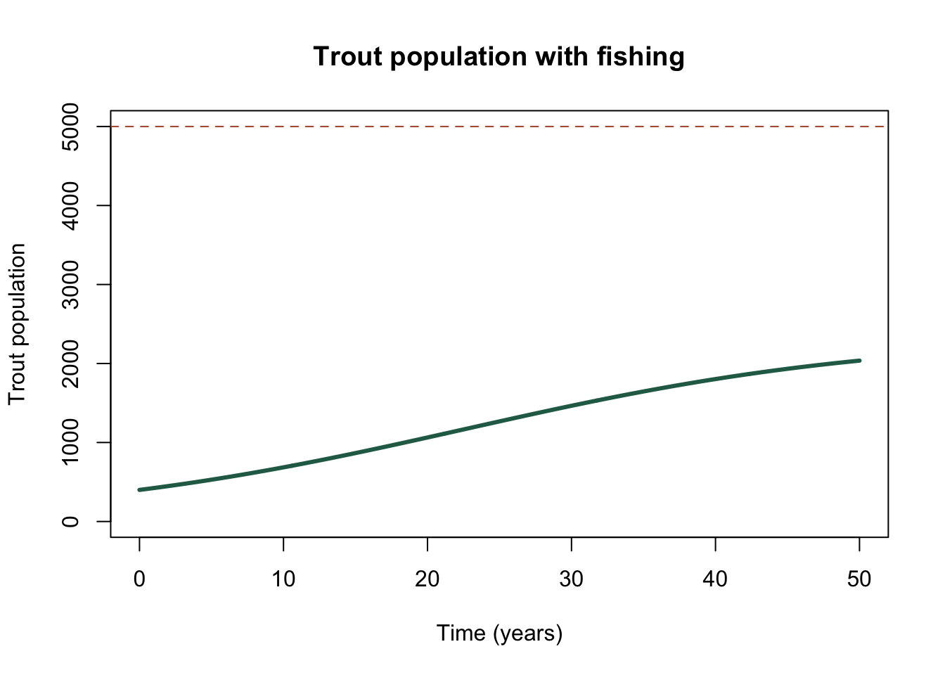

Ask the simulation

When does the population first reach 2,000 trout?

trout_results <- data.frame(
  time = trout_time,
  population = trout_population
)

reach_2000 <- which(trout_results$population >= 2000)[1]
trout_results[c(reach_2000 - 1, reach_2000), ]

        time population
578 48.08333   1999.704
579 48.16667   2001.372

At year 50 the population is still rising. Set the rate of change equal to zero to determine the nonzero long-run equilibrium:

\[ P^*=K\left(1-\frac{f}{r}\right) =5000\left(1-\frac{0.08}{0.15}\right) \approx 2333. \]

The carrying capacity is no longer the equilibrium because fishing adds another outflow.

Change one assumption

Try a fishing rate of 4%, 12%, and 15%. Predict first. Which change affects the speed, and which affects the long-run population?

Problem 2: bacteria during an experiment

A culture begins with 120 bacteria and grows at a continuous rate of 18% per hour. During a 12-hour experiment, assume nutrients are plentiful.

Questions

How many bacteria does the model predict after 12 hours?
When does the culture first exceed 500 bacteria?
How close is the Euler simulation to the analytical solution?

bacteria_delta_t <- 0.25
bacteria_time <- seq(0, 12, by = bacteria_delta_t)
bacteria_rate <- 0.18

bacteria <- numeric(length(bacteria_time))
bacteria[1] <- 120

for (i in 2:length(bacteria_time)) {
  bacteria_old <- bacteria[i - 1]
  growth <- bacteria_rate * bacteria_old
  bacteria[i] <- bacteria_old + growth * bacteria_delta_t
}

bacteria_exact <- 120 * exp(bacteria_rate * bacteria_time)
bacteria_error <- bacteria - bacteria_exact

bacteria_results <- data.frame(
  time = bacteria_time,
  simulated = bacteria,
  exact = bacteria_exact,
  error = bacteria_error
)

tail(bacteria_results)

    time simulated     exact     error
44 10.75  796.4926  830.8853 -34.39270
45 11.00  832.3347  869.1292 -36.79441
46 11.25  869.7898  909.1333 -39.34350
47 11.50  908.9304  950.9788 -42.04842
48 11.75  949.8322  994.7503 -44.91807
49 12.00  992.5747 1040.5365 -47.96185

reach_500 <- which(bacteria_results$simulated >= 500)[1]
bacteria_results[c(reach_500 - 1, reach_500), ]

   time simulated    exact     error
33 8.00  490.7977 506.4835 -15.68577
34 8.25  512.8836 529.7958 -16.91223

plot(
  bacteria_time,
  bacteria,
  type = "l",
  lwd = 3,
  col = "#8b3a3a",
  xlab = "Time (hours)",
  ylab = "Bacteria",
  main = "Unconstrained bacterial growth"
)
lines(bacteria_time, bacteria_exact, lty = 2, lwd = 2)
legend(
  "topleft",
  legend = c("Euler simulation", "Analytical solution"),
  col = c("#8b3a3a", "black"),
  lty = c(1, 2),
  lwd = c(3, 2),
  bty = "n"
)

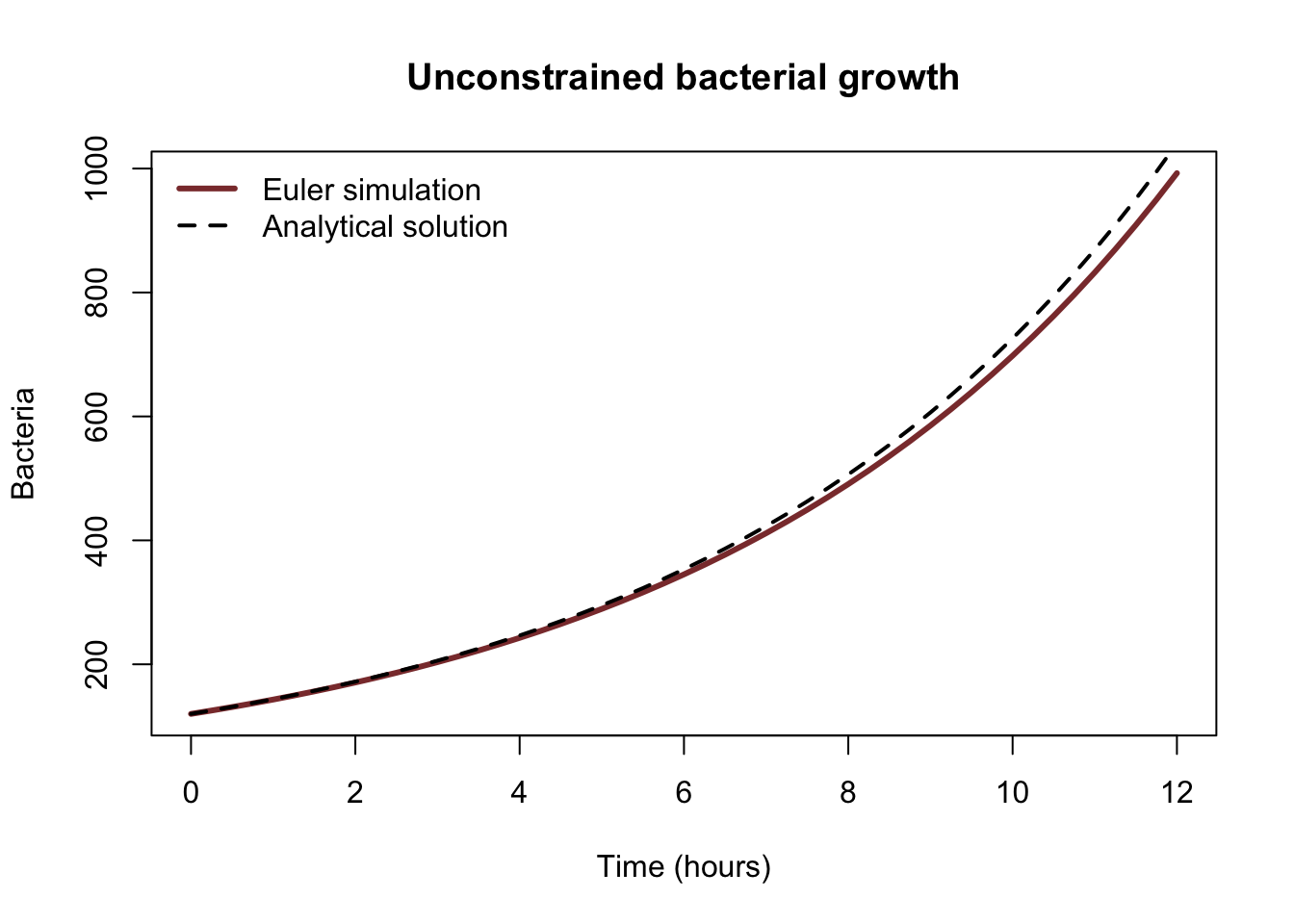
The plentiful-nutrients assumption might be reasonable for 12 hours but unreasonable forever. A model can be useful over one time horizon and poor over another.

Problem 3: caffeine decay

A drink contributes 200 mg of caffeine. Assume the amount in the body has a half-life of 5 hours.

Convert half-life to a decay rate

For exponential decay,

\[ A(t)=A_0e^{-kt}. \]

The elimination constant is

\[ k=\frac{\ln(2)}{\text{half-life}}. \]

caffeine_half_life <- 5
caffeine_decay_constant <- log(2) / caffeine_half_life

caffeine_delta_t <- 0.25
caffeine_time <- seq(0, 24, by = caffeine_delta_t)

caffeine <- numeric(length(caffeine_time))
caffeine[1] <- 200

for (i in 2:length(caffeine_time)) {
  caffeine_old <- caffeine[i - 1]
  eliminated <- caffeine_decay_constant * caffeine_old
  caffeine[i] <- caffeine_old - eliminated * caffeine_delta_t
}

caffeine_results <- data.frame(
  time = caffeine_time,
  caffeine = caffeine
)

below_50 <- which(caffeine_results$caffeine <= 50)[1]
caffeine_results[c(below_50 - 1, below_50), ]

    time caffeine
40  9.75 50.53684
41 10.00 48.78537

plot(
  caffeine_time,
  caffeine,
  type = "l",
  lwd = 3,
  col = "#6b4c8a",
  xlab = "Time (hours)",
  ylab = "Caffeine (mg)",
  main = "Unconstrained decay"
)
abline(h = 50, lty = 2, col = "#b65335")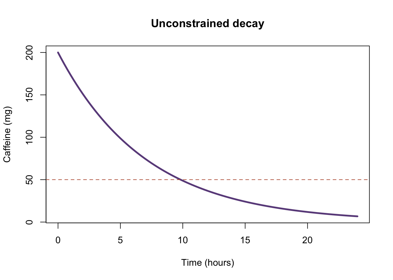

Check without code

After one half-life, 200 mg becomes 100 mg. After two half-lives, it becomes 50 mg. Therefore, the threshold should occur near 10 hours. This rough calculation is an important verification check.

Problem 4: a recovering forest

A recovering forest begins with a biomass index of 80. Its estimated carrying capacity is 1,200, and its unconstrained growth rate is 12% per year.

Predict

Is unconstrained or constrained growth more appropriate over an 80-year period?
At approximately what biomass should growth be fastest?
Will the forest ever reach exactly 1,200 in a finite simulation?

Check the first step by hand

Use a quarterly time step, so \(\Delta t=0.25\) year. At the beginning,

\[ \text{growth rate} =0.12(80)\left(1-\frac{80}{1200}\right) =8.96 \]

biomass-index units per year. Therefore,

\[ P_{new}=80+(8.96)(0.25)=82.24. \]

Build the simulation

forest_delta_t <- 0.25
forest_time <- seq(0, 80, by = forest_delta_t)
forest_growth_rate <- 0.12
forest_capacity <- 1200

forest_biomass <- numeric(length(forest_time))
forest_biomass[1] <- 80

for (i in 2:length(forest_time)) {
  biomass_old <- forest_biomass[i - 1]
  constraint <- 1 - biomass_old / forest_capacity
  growth <- forest_growth_rate * biomass_old * constraint

  forest_biomass[i] <- biomass_old + growth * forest_delta_t
}

forest_results <- data.frame(
  time = forest_time,
  biomass = forest_biomass
)

forest_results$growth <- forest_growth_rate *
  forest_results$biomass *
  (1 - forest_results$biomass / forest_capacity)

head(forest_results)

  time  biomass    growth
1 0.00 80.00000  8.960000
2 0.25 82.24000  9.192458
3 0.50 84.53811  9.429904
4 0.75 86.89559  9.672387
5 1.00 89.31369  9.919949
6 1.25 91.79367 10.172633

The second row should contain 82.24, matching the hand calculation.

Graph the recovery

plot(
  forest_time,
  forest_biomass,
  type = "l",
  lwd = 3,
  col = "#276b55",
  ylim = c(0, forest_capacity * 1.05),
  xlab = "Time (years)",
  ylab = "Biomass index",
  main = "Recovery of forest biomass"
)
abline(h = forest_capacity, lty = 2, col = "#b65335")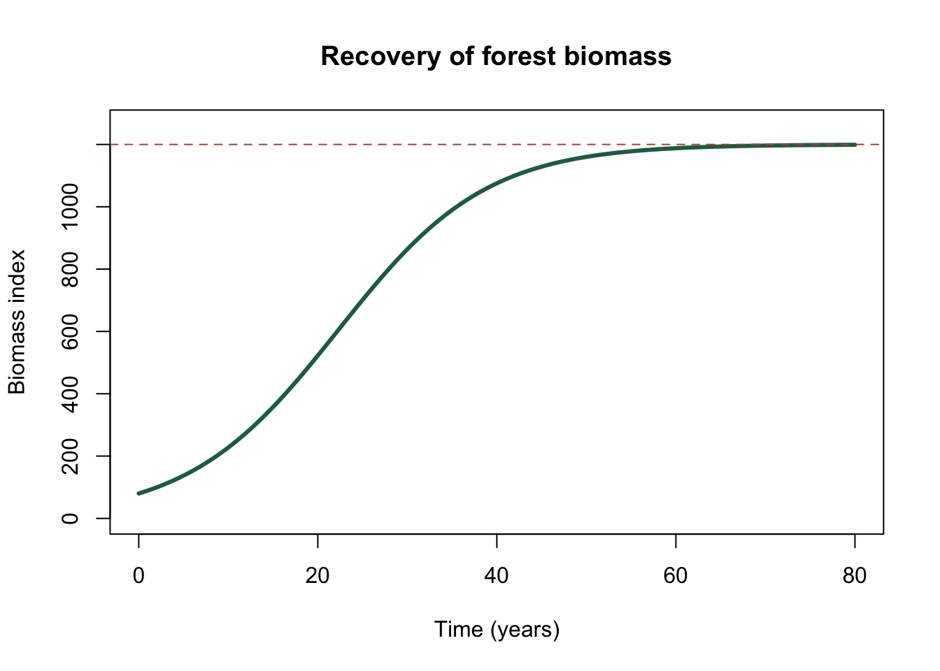

Ask the simulation

When does the forest first reach 75% of carrying capacity?

forest_target <- 0.75 * forest_capacity
reach_forest_target <- which(
  forest_results$biomass >= forest_target
)[1]

forest_results[c(reach_forest_target - 1, reach_forest_target), ]

     time  biomass   growth
126 31.25 899.0371 27.05768
127 31.50 905.8015 26.64854

When is the modeled growth flow largest?

fastest_forest_growth <- which(
  forest_results$growth == max(forest_results$growth)
)[1]

forest_results[fastest_forest_growth, ]

    time  biomass   growth
90 22.25 603.0253 35.99908

Growth is fastest near half of carrying capacity, or a biomass index of 600. After that point, the forest continues growing, but resource limitation has the stronger effect.

Question the assumptions

The model assumes a constant carrying capacity and an immediate response to crowding. A real forest may experience fires, drought, changing climate, delayed tree maturation, harvesting, or different growth rates among species and age groups.

What to remember

Identify the mechanism before choosing a model.
Keep rates, amounts, and time units separate.
Use a hand calculation or known value to check the code.
A threshold question requires the first crossing, not merely the final value.
Carrying capacity is an equilibrium only when no additional flows change the balance.
Growth in the logistic model is fastest near half of carrying capacity.
Every result is conditional on the model’s assumptions and chosen time horizon.