How does population growth change when resources become limited—and how can a simple feedback term keep a model from growing forever?
NoteDownload the example
Download the complete R script. It builds the constrained-growth model, graphs the population and carrying capacity, and answers two questions about the simulation.
Learning goals
After working through this module, you should be able to:
explain why unconstrained growth eventually becomes unrealistic;
interpret carrying capacity and the constraint term;
translate the constrained-growth differential equation into an Euler update;
implement and graph the model in R;
identify equilibria and the region of fastest growth; and
use simulation results to answer threshold questions.
NoteTextbook
Read Module 2.3, “Constrained Growth,” before completing this tutorial.
Begin with a prediction
Suppose a population begins at 20 individuals, grows at 8% per year, and lives in an environment that can support about 500 individuals.
Will the population ever exceed 500?
Will it gain the same number every year?
When will growth be fastest: near 20, near 250, or near 500?
What shape should its graph have?
Add a constraint
The unconstrained model is
\[
\frac{dP}{dt}=rP.
\]
It assumes that the same proportional growth rate continues no matter how large the population becomes. To represent limited food, space, or other resources, introduce a carrying capacity\(K\):
\[
\frac{dP}{dt}=rP\left(1-\frac{P}{K}\right).
\]
Quantity
Meaning
Example units
\(P\)
current population
individuals
\(P_0\)
initial population
individuals
\(r\)
unconstrained proportional growth rate
per year
\(K\)
carrying capacity
individuals
\(t\)
time
years
\(\Delta t\)
length of one simulation step
years
The new factor
\[
1-\frac{P}{K}
\]
measures the fraction of the environment’s capacity that remains available.
Current population
Constraint term
What the model does
\(P\) is small compared with \(K\)
close to 1
behaves almost like unconstrained growth
\(P=K/2\)
\(1/2\)
growth remains positive but is reduced
\(P=K\)
0
population remains constant
\(P>K\)
negative
population decreases toward capacity
ImportantNegative feedback
As the population grows, the constraint term becomes smaller. That reduces the growth flow, which slows further population growth. This balancing feedback is what keeps the model near carrying capacity.
flowchart LR
  R[Growth rate r] --> G[Growth flow]
  P[Population P] --> G
  K[Carrying capacity K] --> C[Constraint 1 - P/K]
  P --> C
  C --> G
  G --> P
flowchart LR
  R[Growth rate r] --> G[Growth flow]
  P[Population P] --> G
  K[Carrying capacity K] --> C[Constraint 1 - P/K]
  P --> C
  C --> G
  G --> P
The Euler update
Over a time step of length \(\Delta t\), approximate the change with
\[
\Delta P \approx rP_{old}\left(1-\frac{P_{old}}{K}\right)\Delta t.
\]
Therefore,
\[
P_{new}=P_{old}+rP_{old}\left(1-\frac{P_{old}}{K}\right)\Delta t.
\]
This is still the same reusable simulation pattern:
\[
\boxed{\text{new amount}=\text{old amount}+\text{rate of change}\times\text{time passed}}
\]
Check one step by hand
Use \(P_{old}=20\), \(r=0.08\) per year, \(K=500\), and \(\Delta t=1\) year.
\[
\text{constraint}=1-\frac{20}{500}=0.96
\]
\[
\text{growth flow}=(0.08)(20)(0.96)=1.536
\]
\[
P_{new}=20+(1.536)(1)=21.536.
\]
Build the simulation in R
1. Define time, parameters, and the initial condition
start_time <-0# yearsend_time <-100# yearsdelta_t <-1# years per stepgrowth_rate <-0.08# per yearcarrying_capacity <-500# individualsinitial_population <-20# individuals
2. Create the time points
time <-seq(from = start_time, to = end_time, by = delta_t)
3. Create and initialize the stock
population <-numeric(length(time))population[1] <- initial_population
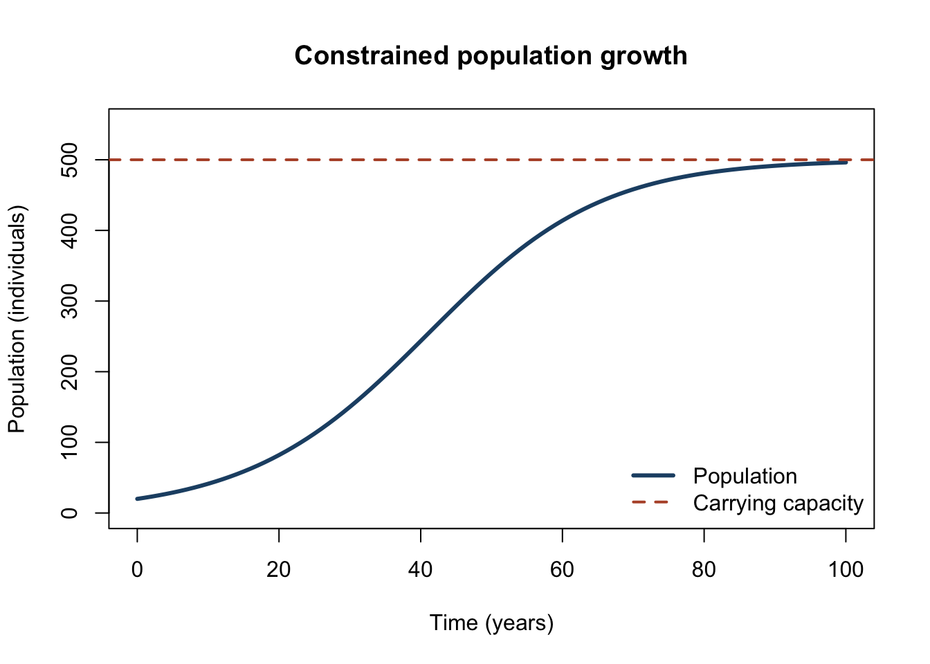
The resulting S-shaped curve is called logistic growth. Growth is initially slow because the population is small, becomes faster as the population increases, and then slows as the population approaches carrying capacity.
   time population constraint   growth
42   41   253.4035  0.4931931 9.998147
For this model, growth is fastest when the population is near \(K/2\). Before that point, adding more individuals increases the total growth flow. After that point, resource limitation has the stronger effect.
Compare with unconstrained growth
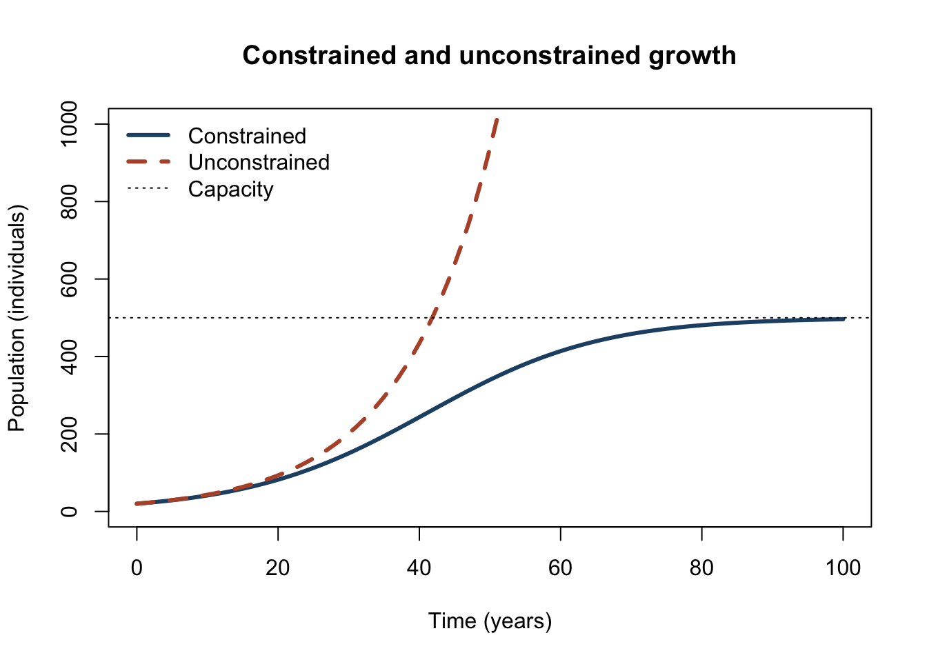
Use the same initial population and growth rate, but remove the constraint:
The unconstrained model eventually exceeds any fixed bound. The constrained model instead approaches an equilibrium near \(K\).
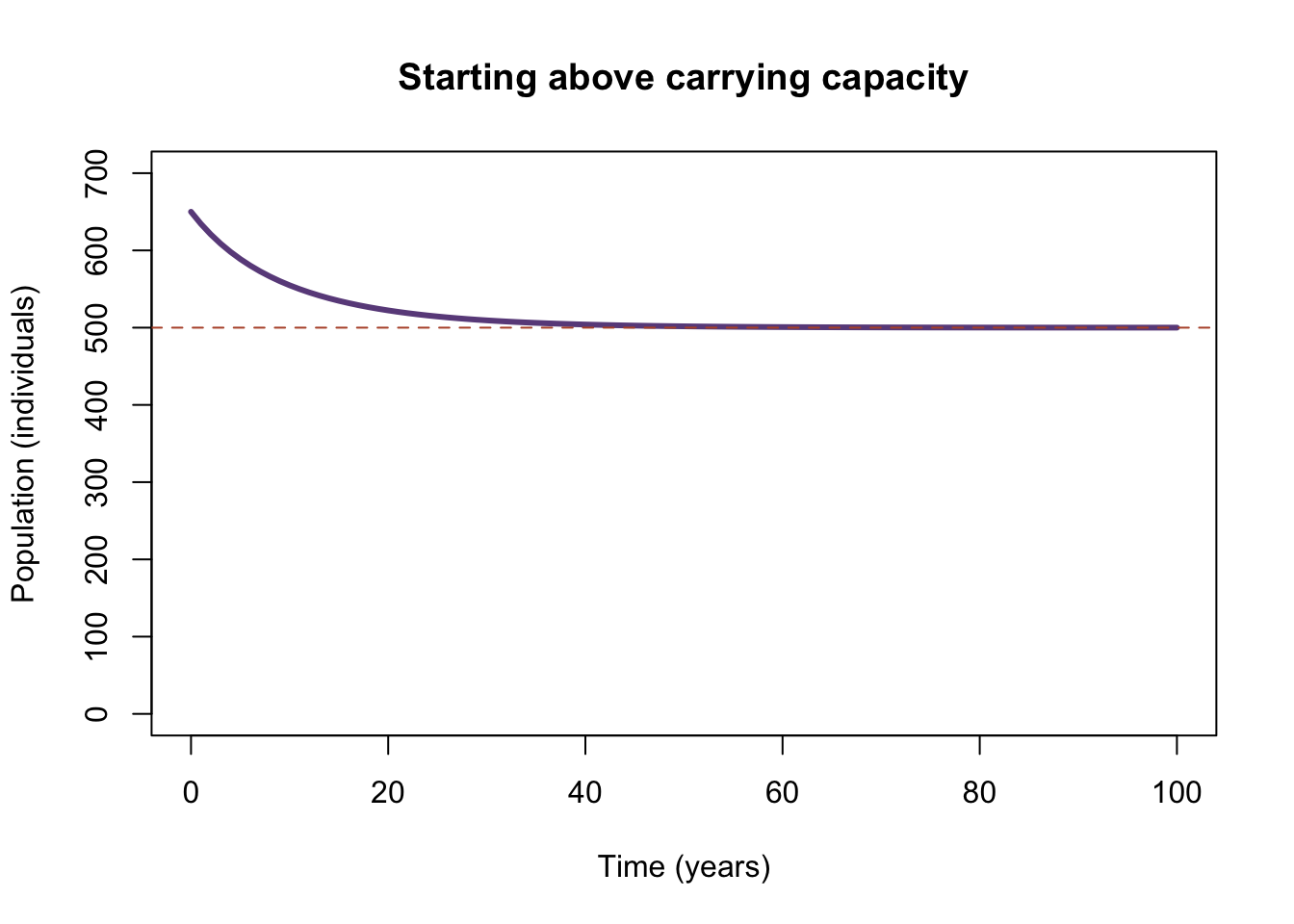
Start above carrying capacity
Carrying capacity is not a wall that the population can never cross. It is an equilibrium toward which the model moves. Test an initial population above capacity:
As in Module 2.2, a smaller time step generally brings the Euler simulation closer to the analytical solution. That verifies the numerical implementation; it does not prove that the model’s assumptions fit a real population.
Assumptions and limits
The constrained-growth model assumes:
carrying capacity remains constant;
the population responds immediately to crowding;
all individuals are interchangeable;
the environment is well mixed;
births and deaths can be represented by continuous rates; and
random events and outside influences are negligible.
Real populations may overshoot a changing capacity, experience delays, migrate, or fluctuate because of seasons and random events. The logistic model is useful because it captures one important feedback—not because it captures everything.
Further experiments
For each experiment, make a prediction before changing the code.
Double the carrying capacity. What changes, and what stays similar?
Double the growth rate. Does the final equilibrium change?
Begin exactly at carrying capacity. What happens?
Begin at population 0. Can the model create individuals from nothing?
Use a very large time step. Can the numerical method overshoot or behave strangely?
Find when the population first reaches 50%, 75%, and 95% of capacity.
What to remember
Carrying capacity represents a sustainable equilibrium, not an impenetrable ceiling.
The constraint \(1-P/K\) weakens growth as the population increases.
Constrained growth uses the same Euler pattern as unconstrained growth.
Growth is fastest near half of carrying capacity.
Populations below or above capacity move toward \(K\) in this model.
Numerical accuracy and model realism are different questions.