flowchart LR
  R[Growth rate r] --> G[Growth flow rP]
  P[Population P] --> G
  G --> P
flowchart LR R[Growth rate r] --> G[Growth flow rP] P[Population P] --> G G --> P
After working through this module, you should be able to:
A population begins with 100 individuals and grows at a continuous rate of 10% per hour.
Keep your predictions. We will test them after building the model.
Let \(P(t)\) be the population at time \(t\) and let \(r\) be its per-capita growth rate. Our central assumption is:
The population’s rate of change is proportional to the population currently present.
Mathematically,
\[ \frac{dP}{dt}=rP. \]
| Quantity | Meaning | Example units |
|---|---|---|
| \(P\) | current population | individuals |
| \(P_0\) | initial population | individuals |
| \(r\) | proportional growth rate | per hour |
| \(t\) | time | hours |
| \(\Delta t\) | length of one simulation step | hours |
The population is a stock: an amount accumulated over time. Growth is a flow into that stock. Because the flow \(rP\) depends on the stock itself, this is a positive feedback loop.
flowchart LR
  R[Growth rate r] --> G[Growth flow rP]
  P[Population P] --> G
G --> Pflowchart LR R[Growth rate r] --> G[Growth flow rP] P[Population P] --> G G --> P
Over a short interval, approximate the derivative with
\[ \frac{P_{new}-P_{old}}{\Delta t}\approx rP_{old}. \]
Solving for the new population gives Euler’s update rule:
\[ P_{new}=P_{old}+rP_{old}\Delta t. \]
This has a form we will reuse throughout the course:
\[ \boxed{\text{new amount}=\text{old amount}+\text{rate of change}\times\text{time passed}} \]
With \(P_{old}=100\), \(r=0.10\) per hour, and \(\Delta t=1\) hour,
\[ P_{new}=100+(0.10)(100)(1)=110. \]
The next increase will be larger because the growth flow is calculated from a larger population.
start_time <- 0             # hours
end_time <- 8               # hours
delta_t <- 1                # hours per step

growth_rate <- 0.10         # per hour
initial_population <- 100   # individuals
Keeping units in the comments makes it easier to catch mistakes.
time <- seq(from = start_time, to = end_time, by = delta_t)
time
[1] 0 1 2 3 4 5 6 7 8Time begins at 0, but R begins counting vector positions at 1. Therefore time[1] contains 0.
population <- numeric(length(time))
population[1] <- initial_population
The vector will store the population’s entire trajectory. Initially, we know only its first value.
for (i in 2:length(time)) {
  population_old <- population[i - 1]
  growth <- growth_rate * population_old
  change <- growth * delta_t

  population[i] <- population_old + change
}
Each iteration reads the previous stock, calculates its flow, converts the flow into a change, and stores the next stock value.
results <- data.frame(time, population)
results
time population
1 0 100.0000
2 1 110.0000
3 2 121.0000
4 3 133.1000
5 4 146.4100
6 5 161.0510
7 6 177.1561
8 7 194.8717
9 8 214.3589Before trusting a graph, verify that the first two rows agree with the hand calculation: 100 at time 0 and 110 at time 1.
plot(
  results$time,
  results$population,
  type = "l",
  lwd = 3,
  col = "#8b3a3a",
  xlab = "Time (hours)",
  ylab = "Population (individuals)",
  main = "Unconstrained population growth"
)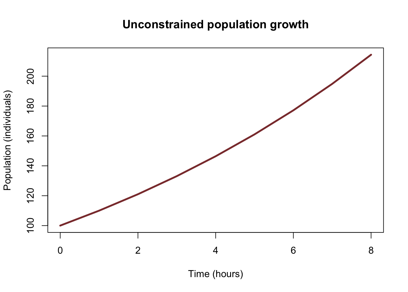
Return to your opening predictions. The curve bends upward because every increase creates a larger population—and therefore an even larger future increase.
Calculus gives the exact solution to this differential equation:
\[ P(t)=P_0e^{rt}. \]
Calculate exact values at the same times and measure the numerical error:
results$exact <- initial_population * exp(growth_rate * results$time)
results$error <- results$population - results$exact
results
time population exact error
1 0 100.0000 100.0000 0.0000000
2 1 110.0000 110.5171 -0.5170918
3 2 121.0000 122.1403 -1.1402758
4 3 133.1000 134.9859 -1.8858808
5 4 146.4100 149.1825 -2.7724698
6 5 161.0510 164.8721 -3.8211271
7 6 177.1561 182.2119 -5.0557800
8 7 194.8717 201.3753 -6.5035607
9 8 214.3589 222.5541 -8.1952118plot(
results$time,
results$exact,
type = "l",
lwd = 3,
col = "#214f73",
xlab = "Time (hours)",
ylab = "Population (individuals)",
main = "Euler simulation and analytical solution"
)
lines(results$time, results$population, lwd = 3, lty = 2, col = "#b65335")
legend(
"topleft",
legend = c("Analytical solution", "Euler simulation"),
col = c("#214f73", "#b65335"),
lty = c(1, 2),
lwd = 3,
bty = "n"
)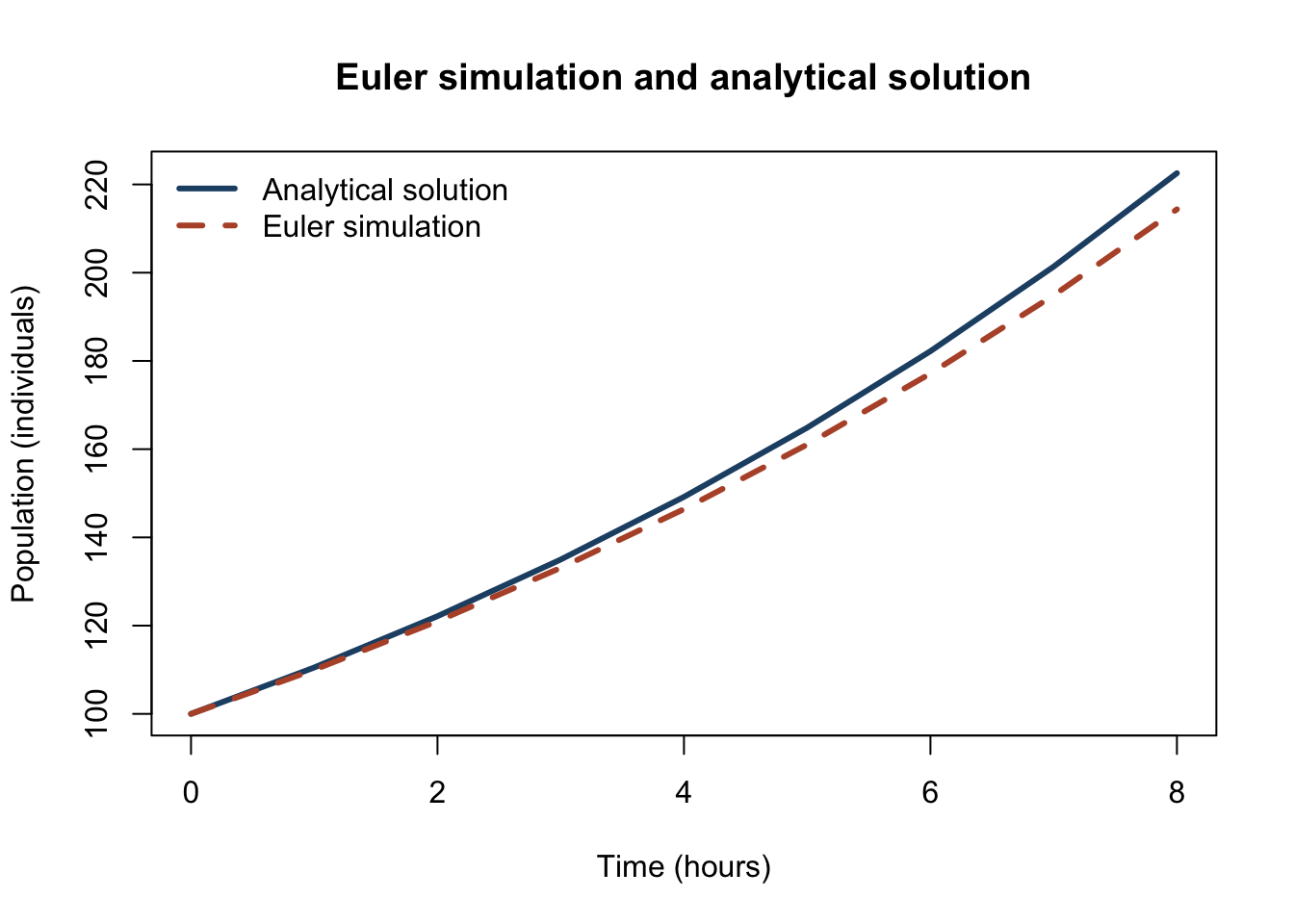
The code can correctly implement Euler’s method without producing the exact continuous solution. The difference is numerical error caused by replacing continuous change with discrete steps.
Run the same model again with a smaller time step. We will use new object names so that we can compare the two simulations.
small_delta_t <- 0.25
small_time <- seq(from = start_time, to = end_time, by = small_delta_t)

small_population <- numeric(length(small_time))
small_population[1] <- initial_population

for (i in 2:length(small_time)) {
  population_old <- small_population[i - 1]
  growth <- growth_rate * population_old
  change <- growth * small_delta_t

  small_population[i] <- population_old + change
}

small_results <- data.frame(
  time = small_time,
  population = small_population
)

small_results$exact <- initial_population *
  exp(growth_rate * small_results$time)
small_results$error <- small_results$population - small_results$exact
Compare the final values from the original one-hour simulation and the new quarter-hour simulation:
exact_at_end <- initial_population * exp(growth_rate * end_time)

data.frame(
  delta_t = c(delta_t, small_delta_t),
  number_of_steps = c(length(time) - 1, length(small_time) - 1),
  final_population = c(
    tail(results$population, 1),
    tail(small_results$population, 1)
  ),
  absolute_error = c(
    abs(tail(results$population, 1) - exact_at_end),
    abs(tail(small_results$population, 1) - exact_at_end)
  )
)
delta_t number_of_steps final_population absolute_error
1 1.00 8 214.3589 8.195212
2 0.25 32 220.3757 2.178399A smaller time step generally reduces Euler error because the rate is recalculated more often. It also requires more computation. Accuracy is therefore connected to both the numerical method and the time-step choice.
The same equation describes decay when \(r<0\). No new algorithm is needed; changing the sign changes the system’s behavior.
decay_start <- 100
decay_rate <- -0.10
decay_end_time <- 20
decay_delta_t <- 0.5

decay_time <- seq(from = 0, to = decay_end_time, by = decay_delta_t)
decay_amount <- numeric(length(decay_time))
decay_amount[1] <- decay_start

for (i in 2:length(decay_time)) {
  amount_old <- decay_amount[i - 1]
  decay_flow <- decay_rate * amount_old
  change <- decay_flow * decay_delta_t

  decay_amount[i] <- amount_old + change
}

decay_results <- data.frame(
  time = decay_time,
  amount = decay_amount
)

decay_results$exact <- decay_start *
exp(decay_rate * decay_results$time)plot(
decay_results$time,
decay_results$exact,
type = "l",
lwd = 3,
col = "#214f73",
xlab = "Time (hours)",
ylab = "Amount",
main = "Unconstrained decay"
)
lines(
decay_results$time,
decay_results$amount,
lwd = 3,
lty = 2,
col = "#b65335"
)
legend(
"topright",
legend = c("Analytical solution", "Euler simulation"),
col = c("#214f73", "#b65335"),
lty = c(1, 2),
lwd = 3,
bty = "n"
)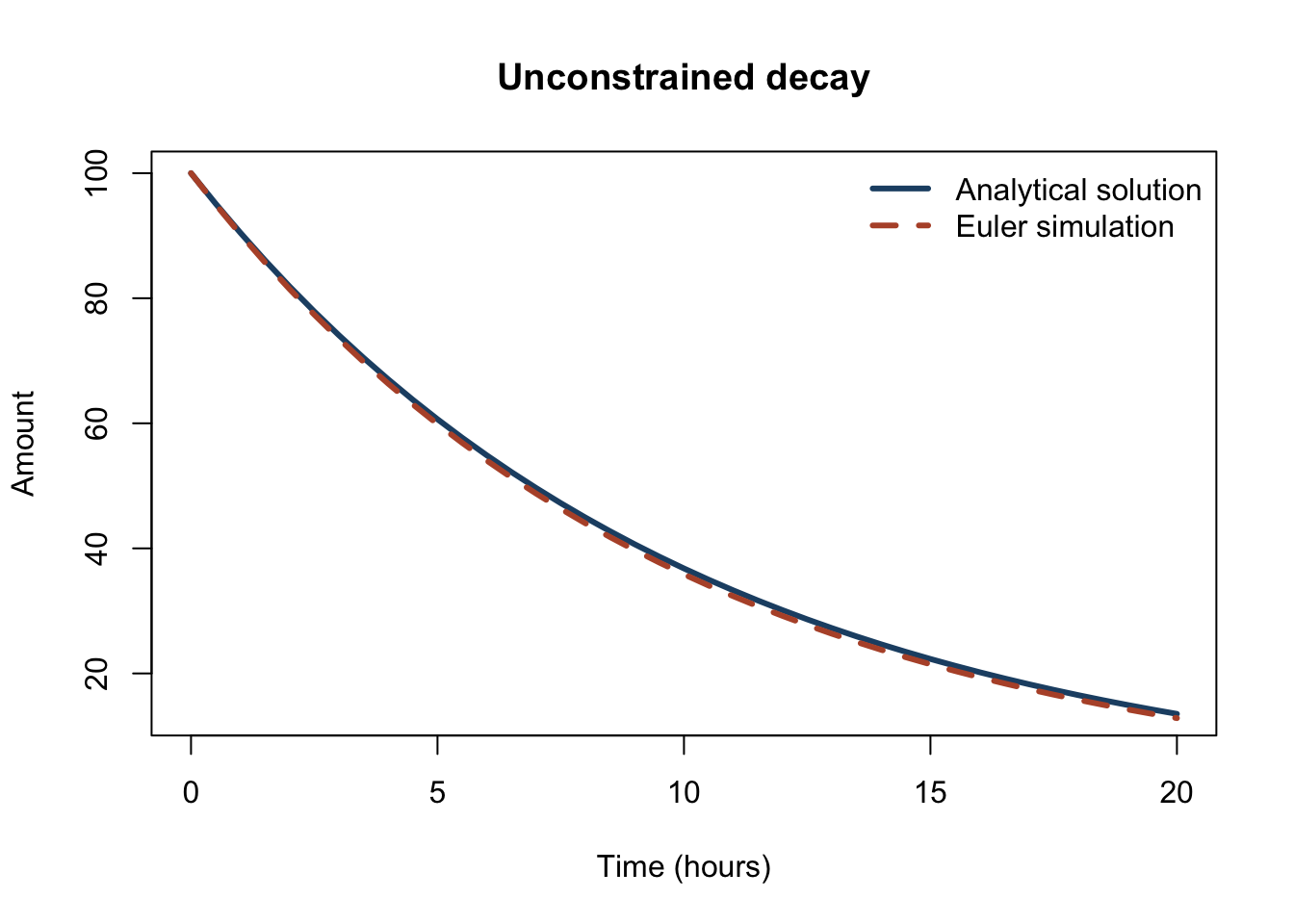
The exact decay curve approaches zero without reaching it. Euler’s method can produce an impossible negative amount if the time step is too large relative to the decay rate.
A graph helps us understand the overall behavior, but a model should also answer specific questions. Many useful questions ask when a stock first crosses a threshold.
Suppose the population begins at 100, grows at 10% per hour, and we simulate with \(\Delta t=0.25\) hour. We already stored that simulation in small_results.
doubling_positions <- which(small_results$population >= 200)
first_double <- doubling_positions[1]

small_results[c(first_double - 1, first_double), ]
time population exact error
29 7.00 199.6495 201.3753 -1.725769
30 7.25 204.6407 206.4731 -1.832371The first displayed row is still below 200; the next row is the first simulated time at or above 200. Checking both rows confirms that we found the first crossing rather than merely a time after the population doubled.
The analytical solution gives an exact doubling time:
exact_doubling_time <- log(2) / 0.10
exact_doubling_time
[1] 6.931472Why is the simulated answer a multiple of 0.25? What happens to the estimated crossing time if delta_t becomes smaller?
Now begin at 100 and decay at 10% per hour. This could represent a pollutant, a medication, or a radioactive substance over a time interval where a constant proportional rate is reasonable. Use the decay simulation we already created.
below_25_positions <- which(decay_results$amount <= 25)
first_below_25 <- below_25_positions[1]

decay_results[c(first_below_25 - 1, first_below_25), ]
time amount exact
28 13.5 25.03441 25.92403
29 14.0 23.78269 24.65970Compare that result with the exact crossing time:
exact_time_below_25 <- log(25 / 100) / -0.10
exact_time_below_25
[1] 13.86294Use the code to investigate one of these:
Before running the model, predict the answer or direction of the effect. Then report the parameter values, threshold-crossing rows, and an interpretation with units.
This model assumes:
Those assumptions may be useful over a limited interval. A numerically accurate answer can still be a poor prediction if the model’s assumptions do not fit reality.
For each experiment, make a prediction, run the model, and explain what happened.
new = old + rate * time passed.In Saving for a Car, the same update pattern controls three quantities: savings, new-car price, and trade-in value.